 pmdarima
A statistical library designed to fill the void in Python's time series analysis capabilities, including the equivalent of R's auto.arima function.
Top Related Projects

Statsmodels: statistical modeling and econometrics in Python

Tool for producing high quality forecasts for time series data that has multiple seasonality with linear or non-linear growth.

Open source time series library for Python

A Python package for Bayesian forecasting with object-oriented design and probabilistic models under the hood.

A unified framework for machine learning with time series

Lightning ⚡️ fast forecasting with statistical and econometric models.
Quick Overview
pmdarima is a Python library for time series forecasting that brings R's auto.arima functionality to Python. It provides tools for automatic ARIMA model selection, forecasting, and statistical testing, making it easier for data scientists and analysts to work with time series data in Python.
Pros
- Automatic model selection simplifies the ARIMA modeling process
- Includes advanced features like seasonal decomposition and exogenous variables
- Compatible with scikit-learn's API, allowing easy integration with existing ML workflows
- Comprehensive documentation and examples
Cons
- Can be computationally intensive for large datasets
- May not always find the optimal model, especially for complex time series
- Limited to ARIMA-based models, which may not be suitable for all time series problems
- Steeper learning curve compared to simpler forecasting libraries
Code Examples
- Basic ARIMA model fitting and forecasting:
from pmdarima import auto_arima
import numpy as np

# Generate sample data
data = np.random.normal(0, 1, 100)

# Fit ARIMA model
model = auto_arima(data, start_p=1, start_q=1, max_p=5, max_q=5, seasonal=False)

# Make forecasts
forecasts = model.predict(n_periods=10)
- Seasonal decomposition:
from pmdarima.preprocessing import decompose
import pandas as pd

# Load data
data = pd.read_csv('time_series_data.csv', parse_dates=['date'], index_col='date')

# Perform seasonal decomposition
decomposition = decompose(data['value'], 'additive', m=12)
trend, seasonal, residual = decomposition.trend, decomposition.seasonal, decomposition.resid
- ARIMA model with exogenous variables:
from pmdarima import auto_arima
import pandas as pd

# Load data with exogenous variables
data = pd.read_csv('data_with_exog.csv', parse_dates=['date'], index_col='date')

# Fit ARIMA model with exogenous variables
model = auto_arima(data['target'], exogenous=data[['exog1', 'exog2']])

# Forecast with future exogenous values
future_exog = pd.DataFrame({'exog1': [1, 2, 3], 'exog2': [4, 5, 6]})
forecasts = model.predict(n_periods=3, X=future_exog)
Getting Started
To get started with pmdarima, follow these steps:
- Install the library:
pip install pmdarima
- Import the necessary modules:
from pmdarima import auto_arima
import pandas as pd
import matplotlib.pyplot as plt
- Load your time series data and fit a model:
data = pd.read_csv('your_data.csv', parse_dates=['date'], index_col='date')
model = auto_arima(data['value'], seasonal=True, m=12)
- Make forecasts and plot the results:
forecasts = model.predict(n_periods=24)
plt.plot(data.index, data['value'], label='Observed')
plt.plot(pd.date_range(start=data.index[-1], periods=25, freq='M')[1:], forecasts, label='Forecast')
plt.legend()
plt.show()
Competitor Comparisons
Statsmodels: statistical modeling and econometrics in Python
Pros of statsmodels
- Comprehensive statistical library with a wide range of models and tests
- Well-established and extensively documented
- Integrates seamlessly with other scientific Python libraries
Cons of statsmodels
- Steeper learning curve for beginners
- Can be slower for certain operations compared to specialized libraries
- Less focused on time series analysis specifically
Code Comparison
statsmodels:
import statsmodels.api as sm
model = sm.tsa.ARIMA(data, order=(1,1,1))
results = model.fit()
forecast = results.forecast(steps=5)
pmdarima:
from pmdarima import auto_arima
model = auto_arima(data, start_p=1, start_q=1, max_p=5, max_q=5)
forecast = model.predict(n_periods=5)
Key Differences
- statsmodels offers a broader range of statistical models and tests
- pmdarima focuses specifically on time series analysis and forecasting
- pmdarima provides automated model selection with auto_arima
- statsmodels requires manual specification of ARIMA parameters
- pmdarima has a more user-friendly API for time series tasks
Both libraries have their strengths, with statsmodels being more comprehensive and pmdarima offering specialized time series functionality. The choice between them depends on the specific requirements of your project and your familiarity with time series analysis.
Tool for producing high quality forecasts for time series data that has multiple seasonality with linear or non-linear growth.
Pros of Prophet
- User-friendly interface with automatic handling of seasonality and holidays
- Robust to missing data and outliers
- Supports multiple seasonalities and custom seasonalities
Cons of Prophet
- Less flexible for complex time series patterns
- Can be slower for large datasets
- Limited options for fine-tuning model parameters
Code Comparison
Prophet:
from fbprophet import Prophet
model = Prophet()
model.fit(df)
future = model.make_future_dataframe(periods=365)
forecast = model.predict(future)
pmdarima:
from pmdarima import auto_arima
model = auto_arima(y, seasonal=True, m=12)
forecast = model.predict(n_periods=365)
Key Differences
- Prophet focuses on ease of use and automatic forecasting
- pmdarima offers more control over model selection and parameters
- Prophet handles seasonality and holidays out-of-the-box
- pmdarima provides a wider range of ARIMA-based models
Use Cases
Prophet is ideal for:
- Quick forecasting with minimal configuration
- Handling multiple seasonalities and holiday effects
pmdarima is better suited for:
- More complex time series analysis
- Fine-tuning model parameters
- Exploring various ARIMA-based models
Both libraries have their strengths, and the choice depends on the specific requirements of the forecasting task at hand.
Open source time series library for Python
Pros of pyflux
- Offers a wider range of time series models, including ARIMA, GARCH, and state space models
- Provides Bayesian inference capabilities for more robust uncertainty quantification
- Includes built-in plotting functions for easy visualization of results
Cons of pyflux
- Less actively maintained, with fewer recent updates compared to pmdarima
- Documentation is less comprehensive and may be outdated in some areas
- Smaller community and fewer contributors, potentially leading to slower bug fixes and feature additions
Code Comparison
pyflux example:
import pyflux as pf
model = pf.ARIMA(data=df['column'], ar=1, ma=1, integ=1)
result = model.fit()
forecast = model.predict(h=5)
pmdarima example:
from pmdarima import auto_arima
model = auto_arima(df['column'], start_p=1, start_q=1, d=1, max_p=5, max_q=5)
forecast = model.predict(n_periods=5)
Both libraries offer ARIMA modeling capabilities, but pyflux provides a more explicit model specification, while pmdarima's auto_arima function automatically selects the best parameters. pmdarima focuses on ease of use and automation, while pyflux offers more flexibility in model customization.
A Python package for Bayesian forecasting with object-oriented design and probabilistic models under the hood.
Pros of Orbit
- Supports Bayesian modeling for time series forecasting
- Handles multiple seasonality patterns
- Provides built-in visualization tools for model diagnostics
Cons of Orbit
- Steeper learning curve due to its Bayesian approach
- More computationally intensive, especially for large datasets
- Less extensive documentation compared to pmdarima
Code Comparison
pmdarima example:
from pmdarima import auto_arima

model = auto_arima(y, seasonal=True, m=12)
forecast = model.predict(n_periods=12)
Orbit example:
from orbit.models import DLT

model = DLT(response_col='y', date_col='ds', seasonality=52)
model.fit(df)
prediction = model.predict(df)
Key Differences
- pmdarima focuses on traditional ARIMA models, while Orbit emphasizes Bayesian structural time series
- Orbit offers more flexibility in modeling complex seasonality patterns
- pmdarima provides automated model selection (auto_arima), whereas Orbit requires more manual configuration
- Orbit integrates well with Pandas DataFrames, while pmdarima works primarily with numpy arrays
Both libraries have their strengths, with pmdarima being more accessible for beginners and Orbit offering advanced capabilities for complex time series modeling.
A unified framework for machine learning with time series
Pros of sktime
- Broader scope: Covers various time series tasks beyond forecasting, including classification and regression
- Scikit-learn compatible: Integrates well with the scikit-learn ecosystem
- Extensive functionality: Offers a wide range of algorithms and tools for time series analysis
Cons of sktime
- Steeper learning curve: More complex API due to its broader scope
- Less specialized: May not offer as deep functionality for specific ARIMA-related tasks
Code Comparison
sktime example:
from sktime.forecasting.arima import ARIMA
forecaster = ARIMA(order=(1, 1, 1), seasonal_order=(1, 1, 1, 12))
forecaster.fit(y_train)
y_pred = forecaster.predict(fh=[1, 2, 3])
pmdarima example:
from pmdarima import auto_arima
model = auto_arima(y_train, seasonal=True, m=12)
forecasts = model.predict(n_periods=3)
The main difference is that pmdarima offers automatic ARIMA model selection with auto_arima, while sktime requires manual specification of ARIMA parameters. However, sktime provides a more consistent interface across different time series tasks and algorithms.
Lightning ⚡️ fast forecasting with statistical and econometric models.
Pros of statsforecast
- Faster execution times, especially for large datasets
- Supports a wider range of statistical forecasting models
- Designed for scalability and high-performance computing
Cons of statsforecast
- Less mature and potentially less stable than pmdarima
- May have a steeper learning curve for users familiar with pmdarima
- Documentation might not be as comprehensive as pmdarima's
Code Comparison
statsforecast:
from statsforecast import StatsForecast
from statsforecast.models import AutoARIMA

sf = StatsForecast(models=[AutoARIMA()], freq='D')
sf.fit(df)
forecasts = sf.predict(h=30)
pmdarima:
from pmdarima import auto_arima

model = auto_arima(y, seasonal=True, m=12)
forecasts = model.predict(n_periods=30)
Both libraries offer AutoARIMA functionality, but statsforecast is designed for handling multiple time series simultaneously, while pmdarima focuses on single time series analysis. statsforecast's API is more oriented towards batch processing, which can be advantageous for large-scale forecasting tasks. However, pmdarima's syntax might be more intuitive for users familiar with traditional statistical modeling approaches.
Convert  designs to code with AI

Introducing Visual Copilot: A new AI model to turn Figma designs to high quality code using your components.
Try Visual CopilotREADME
pmdarima
![]()

![]()
![]()
![]()
Pmdarima (originally pyramid-arima, for the anagram of 'py' + 'arima') is a statistical
library designed to fill the void in Python's time series analysis capabilities. This includes:
- The equivalent of R's
auto.arimafunctionality - A collection of statistical tests of stationarity and seasonality
- Time series utilities, such as differencing and inverse differencing
- Numerous endogenous and exogenous transformers and featurizers, including Box-Cox and Fourier transformations
- Seasonal time series decompositions
- Cross-validation utilities
- A rich collection of built-in time series datasets for prototyping and examples
- Scikit-learn-esque pipelines to consolidate your estimators and promote productionization
Pmdarima wraps statsmodels under the hood, but is designed with an interface that's familiar to users coming from a scikit-learn background.
Installation
pip
Pmdarima has binary and source distributions for Windows, Mac and Linux (manylinux) on pypi
under the package name pmdarima and can be downloaded via pip:
pip install pmdarima
conda
Pmdarima also has Mac and Linux builds available via conda and can be installed like so:
conda config --add channels conda-forge
conda config --set channel_priority strict
conda install pmdarima
Note: We do not maintain our own Conda binaries, they are maintained at https://github.com/conda-forge/pmdarima-feedstock. See that repo for further documentation on working with Pmdarima on Conda.
Quickstart Examples
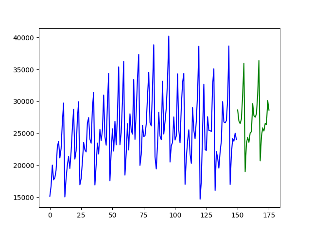
Fitting a simple auto-ARIMA on the wineind dataset:
import pmdarima as pm
from pmdarima.model_selection import train_test_split
import numpy as np
import matplotlib.pyplot as plt

# Load/split your data
y = pm.datasets.load_wineind()
train, test = train_test_split(y, train_size=150)

# Fit your model
model = pm.auto_arima(train, seasonal=True, m=12)

# make your forecasts
forecasts = model.predict(test.shape[0])  # predict N steps into the future

# Visualize the forecasts (blue=train, green=forecasts)
x = np.arange(y.shape[0])
plt.plot(x[:150], train, c='blue')
plt.plot(x[150:], forecasts, c='green')
plt.show()
Fitting a more complex pipeline on the sunspots dataset,
serializing it, and then loading it from disk to make predictions:
import pmdarima as pm
from pmdarima.model_selection import train_test_split
from pmdarima.pipeline import Pipeline
from pmdarima.preprocessing import BoxCoxEndogTransformer
import pickle

# Load/split your data
y = pm.datasets.load_sunspots()
train, test = train_test_split(y, train_size=2700)

# Define and fit your pipeline
pipeline = Pipeline([
    ('boxcox', BoxCoxEndogTransformer(lmbda2=1e-6)),  # lmbda2 avoids negative values
    ('arima', pm.AutoARIMA(seasonal=True, m=12,
                           suppress_warnings=True,
                           trace=True))
])

pipeline.fit(train)

# Serialize your model just like you would in scikit:
with open('model.pkl', 'wb') as pkl:
    pickle.dump(pipeline, pkl)

# Load it and make predictions seamlessly:
with open('model.pkl', 'rb') as pkl:
    mod = pickle.load(pkl)
    print(mod.predict(15))
# [25.20580375 25.05573898 24.4263037  23.56766793 22.67463049 21.82231043
# 21.04061069 20.33693017 19.70906027 19.1509862  18.6555793  18.21577243
# 17.8250318  17.47750614 17.16803394]
Availability
pmdarima is available on PyPi in pre-built Wheel files for Python 3.9+ for the following platforms:
- Mac (64-bit)
- Linux (64-bit manylinux)
- Windows (64-bit)
- 32-bit wheels are available for pmdarima versions below 2.0.0 and Python versions below 3.10
If a wheel doesn't exist for your platform, you can still pip install and it
will build from the source distribution tarball, however you'll need cython>=0.29
and gcc (Mac/Linux) or MinGW (Windows) in order to build the package from source.
Note that legacy versions (<1.0.0) are available under the name
"pyramid-arima" and can be pip installed via:
# Legacy warning:
$ pip install pyramid-arima
# python -c 'import pyramid;'
However, this is not recommended.
Documentation
All of your questions and more (including examples and guides) can be answered by
the pmdarima documentation. If not, always
feel free to file an issue.
Top Related Projects
Statsmodels: statistical modeling and econometrics in Python
Tool for producing high quality forecasts for time series data that has multiple seasonality with linear or non-linear growth.
Open source time series library for Python
A Python package for Bayesian forecasting with object-oriented design and probabilistic models under the hood.
A unified framework for machine learning with time series
Lightning ⚡️ fast forecasting with statistical and econometric models.
Convert designs to code with AI
Introducing Visual Copilot: A new AI model to turn Figma designs to high quality code using your components.
Try Visual Copilot