CMC

[arXiv 2019] "Contrastive Multiview Coding", also contains implementations for MoCo and InstDis

1,298

179

1,298

View on GitHub

Top Related Projects

pytorch-metric-learning

5,939

The easiest way to use deep metric learning in your application. Modular, flexible, and extensible. Written in PyTorch.

moco

4,714

PyTorch implementation of MoCo: https://arxiv.org/abs/1911.05722

swav

1,988

PyTorch implementation of SwAV https//arxiv.org/abs/2006.09882

simclr

4,047

SimCLRv2 - Big Self-Supervised Models are Strong Semi-Supervised Learners

lightly

2,918

A python library for self-supervised learning on images.

Quick Overview

CMC (Contrastive Multiview Coding) is a self-supervised learning framework for visual representations. It leverages multiple views of the data to learn robust and transferable features without relying on labeled data. The project implements the CMC approach as described in the paper "Contrastive Multiview Coding" by Yonglong Tian, Dilip Krishnan, and Phillip Isola.

Pros

Effective self-supervised learning method for visual representations
Utilizes multiple views of data to learn more robust features
Achieves competitive performance on various downstream tasks
Provides a PyTorch implementation for easy experimentation and integration

Cons

Limited documentation and examples for newcomers
May require significant computational resources for training on large datasets
Focused primarily on image data, potentially limiting its applicability to other domains
Requires careful hyperparameter tuning for optimal performance

Code Examples

Loading a pre-trained CMC model:

from models.alexnet import alexnet

# Load pre-trained CMC model
model = alexnet(feat_dim=128)
checkpoint = torch.load('path/to/checkpoint.pth.tar', map_location='cpu')
model.load_state_dict(checkpoint['model'])

Extracting features using a CMC model:

import torch

# Assume 'model' is a loaded CMC model
model.eval()

# Prepare input data (assuming normalized image tensor)
input_tensor = torch.randn(1, 3, 224, 224)

# Extract features
with torch.no_grad():
    features = model(input_tensor)

Training a CMC model:

from models.alexnet import alexnet
from NCE.NCEAverage import NCEAverage
from NCE.NCECriterion import NCECriterion

# Initialize model and NCE components
model = alexnet(feat_dim=128)
contrast = NCEAverage(128, n_data, args.nce_k, args.nce_t, args.nce_m)
criterion = NCECriterion(n_data)

# Training loop (simplified)
for epoch in range(num_epochs):
    for images, _ in train_loader:
        feat_l, feat_ab = model(images)
        out_l, out_ab = contrast(feat_l, feat_ab)
        loss = criterion(out_l) + criterion(out_ab)
        
        optimizer.zero_grad()
        loss.backward()
        optimizer.step()

Getting Started

To get started with CMC:

Clone the repository:

git clone https://github.com/HobbitLong/CMC.git
cd CMC

Install dependencies:
```
pip install -r requirements.txt
```
Prepare your dataset and modify the configuration in config.py.

Run training:

python train.py --data_folder /path/to/data --model alexnet --moco_k 4096

Evaluate the trained model:

python linear_eval.py --model_path /path/to/checkpoint.pth.tar

Competitor Comparisons

pytorch-metric-learning

5,939

The easiest way to use deep metric learning in your application. Modular, flexible, and extensible. Written in PyTorch.

Pros of pytorch-metric-learning

More comprehensive library with a wider range of metric learning techniques
Better documentation and examples for easier implementation
Active development and community support

Cons of pytorch-metric-learning

Potentially more complex to use for simple tasks
May have a steeper learning curve for beginners

Code Comparison

CMC:

from CMC import CMC

model = CMC(backbone, feat_dim=128, NCE_k=4096, NCE_t=0.07)
criterion = NCECriterion(4096)
optimizer = optim.SGD(model.parameters(), lr=0.03, momentum=0.9)

pytorch-metric-learning:

from pytorch_metric_learning import losses, miners, distances

loss_func = losses.NTXentLoss(temperature=0.07)
mining_func = miners.MultiSimilarityMiner()
distance = distances.CosineSimilarity()

Both libraries offer implementations for contrastive learning, but pytorch-metric-learning provides more flexibility and options for different loss functions, mining strategies, and distance metrics. CMC focuses specifically on Contrastive Multiview Coding, while pytorch-metric-learning covers a broader range of metric learning techniques.

moco

4,714

PyTorch implementation of MoCo: https://arxiv.org/abs/1911.05722

Pros of MoCo

Larger community support and more extensive documentation
Regularly updated with new features and improvements
Broader applicability across various computer vision tasks

Cons of MoCo

More complex implementation, potentially harder for beginners
Requires more computational resources for training
Less flexibility in terms of contrastive learning approaches

Code Comparison

MoCo:

# MoCo v2 encoder
self.encoder_q = base_encoder(num_classes=dim)
self.encoder_k = base_encoder(num_classes=dim)

for param_q, param_k in zip(self.encoder_q.parameters(), self.encoder_k.parameters()):
    param_k.data.copy_(param_q.data)
    param_k.requires_grad = False

CMC:

# CMC encoder
self.encoder = base_encoder(num_classes=dim)
self.encoder_k = base_encoder(num_classes=dim)

for param_q, param_k in zip(self.encoder.parameters(), self.encoder_k.parameters()):
    param_k.data.copy_(param_q.data)
    param_k.requires_grad = False

Both repositories implement contrastive learning methods for self-supervised visual representation learning. MoCo focuses on momentum contrast, while CMC emphasizes contrastive multiview coding. The code snippets show similarities in encoder initialization, but MoCo's implementation is generally more complex and feature-rich. CMC offers a simpler approach that may be easier for newcomers to understand and implement.

swav

1,988

PyTorch implementation of SwAV https//arxiv.org/abs/2006.09882

Pros of SwAV

More comprehensive and well-documented codebase
Supports multi-crop strategy for improved performance
Implements online clustering for efficient training

Cons of SwAV

Higher computational requirements
More complex implementation, potentially harder to adapt

Code Comparison

SwAV:

class SwAV(nn.Module):
    def __init__(self, base_encoder, dim=128, K=65536, T=0.1, m=0.99, num_crops=2):
        super(SwAV, self).__init__()
        self.K = K
        self.T = T
        self.m = m
        self.num_crops = num_crops
        # ... (additional initialization code)

CMC:

class CMC(nn.Module):
    def __init__(self, base_encoder, dim=128):
        super(CMC, self).__init__()
        self.encoder = base_encoder(num_classes=dim)
        self.head = nn.Sequential(
            nn.Linear(dim, dim),
            nn.ReLU(inplace=True),
            nn.Linear(dim, dim)
        )

SwAV offers a more advanced implementation with features like multi-crop strategy and online clustering, which can lead to better performance. However, this comes at the cost of increased complexity and computational requirements. CMC, on the other hand, provides a simpler implementation that may be easier to understand and adapt, but might not achieve the same level of performance as SwAV in certain scenarios.

simclr

4,047

SimCLRv2 - Big Self-Supervised Models are Strong Semi-Supervised Learners

Pros of SimCLR

More comprehensive documentation and examples
Larger community support and active development
Implements more recent advancements in self-supervised learning

Cons of SimCLR

Higher computational requirements
More complex architecture, potentially harder to understand and modify
Less flexibility in terms of contrastive learning approaches

Code Comparison

SimCLR:

def contrastive_loss(hidden1, hidden2, temperature=1.0):
    hidden1, hidden2 = tf.math.l2_normalize(hidden1, axis=1), tf.math.l2_normalize(hidden2, axis=1)
    batch_size = tf.shape(hidden1)[0]
    labels = tf.range(batch_size)
    masks = tf.one_hot(labels, batch_size)
    logits_aa = tf.matmul(hidden1, hidden1, transpose_b=True) / temperature
    logits_bb = tf.matmul(hidden2, hidden2, transpose_b=True) / temperature
    logits_ab = tf.matmul(hidden1, hidden2, transpose_b=True) / temperature
    return losses.contrastive_loss(labels, logits_ab, masks)

CMC:

def NCE_loss(q, k, neg, T=0.07):
    N = q.shape[0]
    K = k.shape[0]
    q = nn.functional.normalize(q, dim=1)
    k = nn.functional.normalize(k, dim=1)
    neg = nn.functional.normalize(neg, dim=1)
    pos = torch.bmm(q.view(N, 1, -1), k.view(N, -1, 1)).squeeze(-1)
    neg = torch.mm(q, neg.transpose(1, 0))
    logits = torch.cat([pos, neg], dim=1)
    labels = torch.zeros(N, dtype=torch.long).cuda()
    return nn.CrossEntropyLoss()(logits / T, labels)

lightly

2,918

A python library for self-supervised learning on images.

Pros of lightly

More comprehensive framework for self-supervised learning and active learning
Extensive documentation and tutorials for easier adoption
Actively maintained with frequent updates and community support

Cons of lightly

Larger codebase and potentially steeper learning curve
May include features not necessary for all use cases, leading to overhead
Less focused on specific contrastive learning techniques compared to CMC

Code Comparison

CMC (contrastive multiview coding):

class CMC(nn.Module):
    def __init__(self, base_encoder, dim=128, K=65536, m=0.999, T=0.07, mlp=False):
        super(CMC, self).__init__()
        self.K = K
        self.m = m
        self.T = T

lightly (general self-supervised learning framework):

class SimCLR(pl.LightningModule):
    def __init__(self, backbone, num_ftrs, out_dim, num_negatives, temperature):
        super().__init__()
        self.backbone = backbone
        self.projection_head = ProjectionHead(num_ftrs, out_dim)
        self.criterion = NTXentLoss(temperature, num_negatives)

Convert designs to code with AI

Introducing Visual Copilot: A new AI model to turn Figma designs to high quality code using your components.

Try Visual Copilot

README

Official implementation:

CMC: Contrastive Multiview Coding (Paper)

Unofficial implementation:

MoCo: Momentum Contrast for Unsupervised Visual Representation Learning (Paper)
InsDis: Unsupervised Feature Learning via Non-Parametric Instance-level Discrimination (Paper)

Citation

If you find this repo useful for your research, please consider citing the paper

@article{tian2019contrastive,
  title={Contrastive Multiview Coding},
  author={Tian, Yonglong and Krishnan, Dilip and Isola, Phillip},
  journal={arXiv preprint arXiv:1906.05849},
  year={2019}
}

Contrastive Multiview Coding

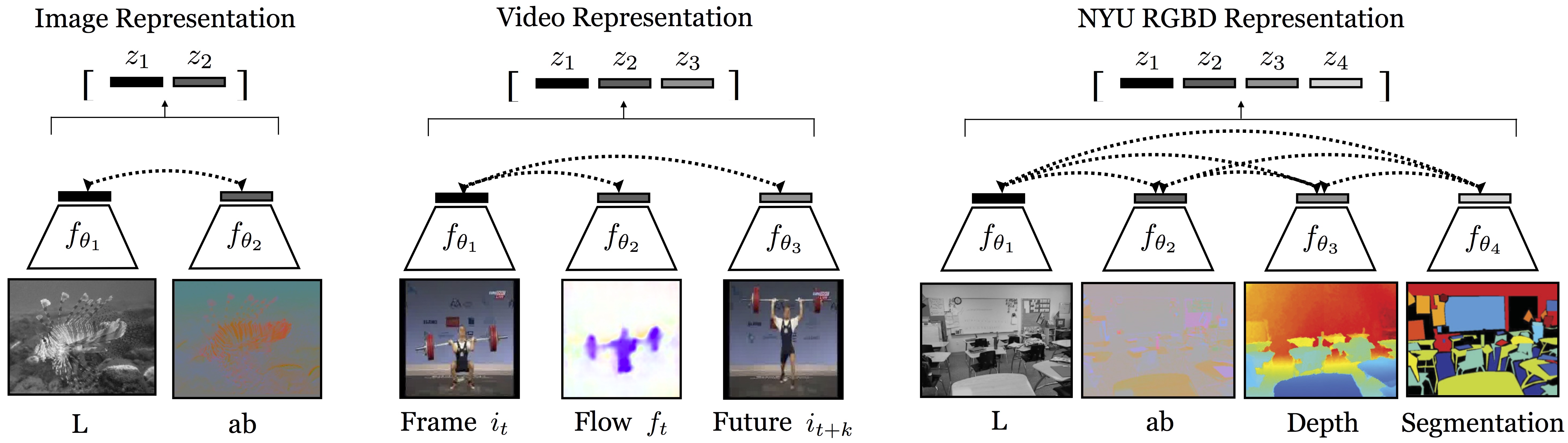
This repo covers the implementation for CMC (as well as Momentum Contrast and Instance Discrimination), which learns representations from multiview data in a self-supervised way (by multiview, we mean multiple sensory, multiple modal data, or literally multiple viewpoint data. It's flexible to define what is a "view"):

"Contrastive Multiview Coding" Paper, Project Page.

Teaser Image

Highlights

(1) Representation quality as a function of number of contrasted views.

We found that, the more views we train with, the better the representation (of each single view).

(2) Contrastive objective v.s. Predictive objective

We compare the contrastive objective to cross-view prediction, finding an advantage to the contrastive approach.

(3) Unsupervised v.s. Supervised

Several ResNets trained with our unsupervised CMC objective surpasses supervisedly trained AlexNet on ImageNet classification ( e.g., 68.4% v.s. 59.3%). For this first time on ImageNet classification, unsupervised methods are surpassing the classic supervised-AlexNet proposed in 2012 (CPC++ and AMDIM also achieve this milestone concurrently).

Updates

Aug 20, 2019 - ResNets on ImageNet have been added.

Nov 26, 2019 - New results updated. Implementation of MoCo and InsDis added.

Jan 18, 2020 - Weights of InsDis and MoCo added.

May 22, 2020 - ImageNet-100 list uploaded, see imagenet100.txt.

Installation

This repo was tested with Ubuntu 16.04.5 LTS, Python 3.5, PyTorch 0.4.0, and CUDA 9.0. But it should be runnable with recent PyTorch versions >=0.4.0

Note: It seems to us that training with Pytorch version >= 1.0 yields slightly worse results. If you find the similar discrepancy and figure out the problem, please report this since we are trying to fix it as well.

Training AlexNet/ResNets with CMC on ImageNet

Note: For AlexNet, we split across the channel dimension and use each half to encode L and ab. For ResNets, we use a standard ResNet model to encode each view.

NCE flags:

--nce_k: number of negatives to contrast for each positive. Default: 4096
--nce_m: the momentum for dynamically updating the memory. Default: 0.5
--nce_t: temperature that modulates the distribution. Default: 0.07 for ImageNet, 0.1 for STL-10

Path flags:

--data_folder: specify the ImageNet data folder.
--model_path: specify the path to save model.
--tb_path: specify where to save tensorboard monitoring events.

Model flag:

--model: specify which model to use, including alexnet, resnets18, resnets50, and resnets101

An example of command line for training CMC (Default: AlexNet on Single GPU)

CUDA_VISIBLE_DEVICES=0 python train_CMC.py --batch_size 256 --num_workers 36 \
 --data_folder /path/to/data 
 --model_path /path/to/save 
 --tb_path /path/to/tensorboard

Training CMC with ResNets requires at least 4 GPUs, the command of using resnet50v1 looks like

CUDA_VISIBLE_DEVICES=0,1,2,3 python train_CMC.py --model resnet50v1 --batch_size 128 --num_workers 24
 --data_folder path/to/data \
 --model_path path/to/save \
 --tb_path path/to/tensorboard \

To support mixed precision training, simply append the flag --amp, which, however is likely to harm the downstream classification. I measure it on ImageNet100 subset and the gap is about 0.5-1%.

By default, the training scripts will use L and ab as two views for contrasting. You can switch to YCbCr by specifying --view YCbCr, which yields better results (about 0.5-1%). If you want to use other color spaces as different views, follow the line here and other color transfer functions are already available in dataset.py.

Training Linear Classifier

Path flags:

--data_folder: specify the ImageNet data folder. Should be the same as above.
--save_path: specify the path to save the linear classifier.
--tb_path: specify where to save tensorboard events monitoring linear classifier training.

Model flag --model is similar as above and should be specified.

Specify the checkpoint that you want to evaluate with --model_path flag, this path should directly point to the .pth file.

This repo provides 3 ways to train the linear classifier: single GPU, data parallel, and distributed data parallel.

An example of command line for evaluating, say ./models/alexnet.pth, should look like:

CUDA_VISIBLE_DEVICES=0 python LinearProbing.py --dataset imagenet \
 --data_folder /path/to/data \
 --save_path /path/to/save \
 --tb_path /path/to/tensorboard \
 --model_path ./models/alexnet.pth \
 --model alexnet --learning_rate 0.1 --layer 5

Note: When training linear classifiers on top of ResNets, it's important to use large learning rate, e.g., 30~50. Specifically, change --learning_rate 0.1 --layer 5 to --learning_rate 30 --layer 6 for resnet50v1 and resnet50v2, to --learning_rate 50 --layer 6 for resnet50v3.

Pretrained Models

Pretrained weights can be found in Dropbox.

Note:

CMC weights are trained with NCE loss, Lab color space, 4096 negatives and amp option. Switching to softmax-ce loss, YCbCr, 65536 negatives, and turning off amp option, are likely to improve the results.
CMC_resnet50v2.pth and CMC_resnet50v3.pth are trained with FastAutoAugment, which improves the downstream accuracy by 0.8~1%. I will update weights without FastAutoAugment once they are available.

InsDis and MoCo are trained using the same hyperparameters as in MoCo (epochs=200, lr=0.03, lr_decay_epochs=120,160, weight_decay=1e-4), but with only 4 GPUs.

	Arch	#Params(M)	Loss	#Negative	Accuracy(%)	Delta(%)
InsDis	ResNet50	24	NCE	4096	56.5	-
InsDis	ResNet50	24	Softmax-CE	4096	57.1	+0.6
InsDis	ResNet50	24	Softmax-CE	16384	58.5	+1.4
MoCo	ResNet50	24	Softmax-CE	16384	59.4	+0.9

Momentum Contrast and Instance Discrimination

I have implemented and tested MoCo and InsDis on a ImageNet100 subset (but the code allows one to train on full ImageNet simply by setting the flag --dataset imagenet):

The pre-training stage:

For InsDis:

CUDA_VISIBLE_DEVICES=0,1,2,3 python train_moco_ins.py \
 --batch_size 128 --num_workers 24 --nce_k 16384 --softmax

For MoCo:

CUDA_VISIBLE_DEVICES=0,1,2,3 python train_moco_ins.py \
 --batch_size 128 --num_workers 24 --nce_k 16384 --softmax --moco

The linear evaluation stage:

For both InsDis and MoCo (lr=10 is better than 30 on this subset, for full imagenet please switch to 30):

CUDA_VISIBLE_DEVICES=0 python eval_moco_ins.py --model resnet50 \
 --model_path /path/to/model --num_workers 24 --learning_rate 10

The comparison of CMC (using YCbCr), MoCo and InsDIS on my ImageNet100 subset, is tabulated as below:

	Arch	#Params(M)	Loss	#Negative	Accuracy
InsDis	ResNet50	24	NCE	16384	--
InsDis	ResNet50	24	Softmax-CE	16384	69.1
MoCo	ResNet50	24	NCE	16384	--
MoCo	ResNet50	24	Softmax-CE	16384	73.4
CMC	2xResNet50half	12	NCE	4096	--
CMC	2xResNet50half	12	Softmax-CE	4096	75.8

For any questions, please contact Yonglong Tian (yonglong@mit.edu).

Acknowledgements

Part of this code is inspired by Zhirong Wu's unsupervised learning algorithm lemniscate.

Top Related Projects

Convert designs to code with AI

Introducing Visual Copilot: A new AI model to turn Figma designs to high quality code using your components.

Try Visual Copilot