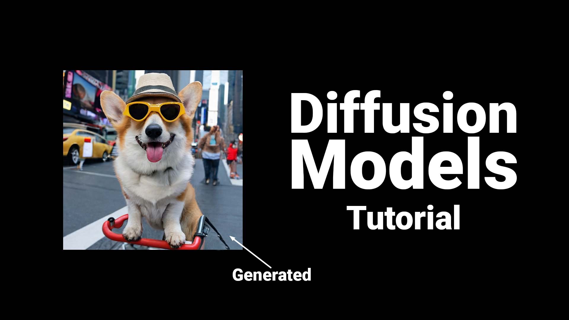
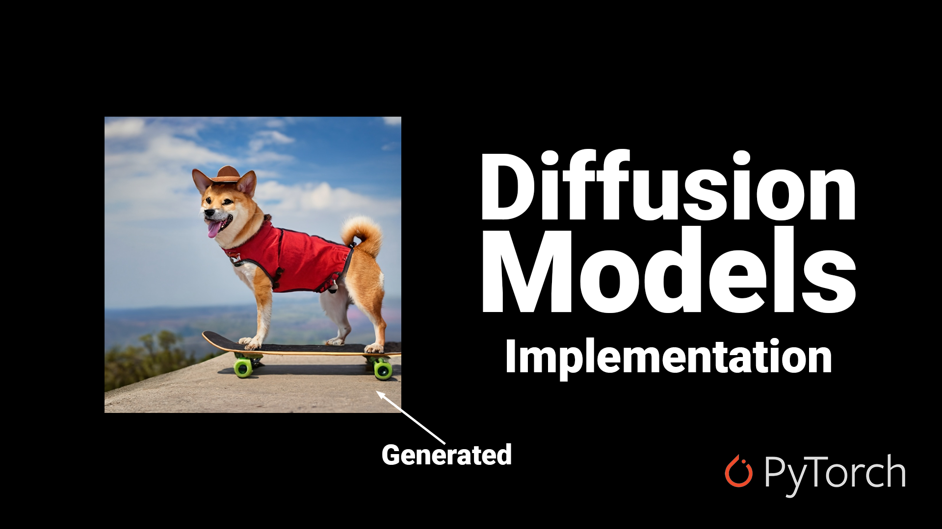
 Diffusion-Models-pytorch
Pytorch implementation of Diffusion Models (https://arxiv.org/pdf/2006.11239.pdf)
Top Related Projects
A latent text-to-image diffusion model
Implementation of Denoising Diffusion Probabilistic Model in Pytorch
Denoising Diffusion Probabilistic Models
Denoising Diffusion Implicit Models
Quick Overview
The dome272/Diffusion-Models-pytorch repository is an implementation of diffusion models in PyTorch. It provides a simple and educational codebase for understanding and experimenting with diffusion models, which are a class of generative models that have gained popularity in recent years for their high-quality image generation capabilities.
Pros
- Clear and concise implementation of diffusion models
- Educational resource for understanding diffusion model concepts
- Includes both training and sampling scripts
- Built with PyTorch, a popular deep learning framework
Cons
- Limited documentation and explanations
- May not include the latest optimizations or techniques in diffusion models
- Focused on a specific dataset (MNIST), which may limit its applicability
- Not actively maintained (last commit over a year ago)
Code Examples
- Defining the UNet model architecture:
class UNet(nn.Module):
    def __init__(self, c_in=1, c_out=1, time_dim=256):
        super().__init__()
        self.time_dim = time_dim
        self.inc = DoubleConv(c_in, 64)
        self.down1 = Down(64, 128)
        self.sa1 = SelfAttention(128, 32)
        self.down2 = Down(128, 256)
        self.sa2 = SelfAttention(256, 16)
        self.down3 = Down(256, 256)
        self.sa3 = SelfAttention(256, 8)

        self.bot1 = DoubleConv(256, 512)
        self.bot2 = DoubleConv(512, 512)
        self.bot3 = DoubleConv(512, 256)

        self.up1 = Up(512, 128)
        self.sa4 = SelfAttention(128, 16)
        self.up2 = Up(256, 64)
        self.sa5 = SelfAttention(64, 32)
        self.up3 = Up(128, 64)
        self.sa6 = SelfAttention(64, 64)
        self.outc = nn.Conv2d(64, c_out, kernel_size=1)
- Implementing the forward pass of the diffusion model:
def forward(self, x, t):
    t = self.pos_encoding(t)
    x1 = self.inc(x)
    x2 = self.down1(x1, t)
    x2 = self.sa1(x2)
    x3 = self.down2(x2, t)
    x3 = self.sa2(x3)
    x4 = self.down3(x3, t)
    x4 = self.sa3(x4)

    x4 = self.bot1(x4)
    x4 = self.bot2(x4)
    x4 = self.bot3(x4)

    x = self.up1(x4, x3, t)
    x = self.sa4(x)
    x = self.up2(x, x2, t)
    x = self.sa5(x)
    x = self.up3(x, x1, t)
    x = self.sa6(x)
    output = self.outc(x)
    return output
- Training loop for the diffusion model:
for epoch in range(args.epochs):
    for step, batch in enumerate(dataloader):
        optimizer.zero_grad()

        t = torch.randint(0, T, (BATCH_SIZE,), device=device).long()
        loss = diffusion.p_losses(model, batch[0], t, loss_type="huber")

        loss.backward()
        optimizer.step()

        if epoch % 10 == 0 and step == 0:
            print(f"Epoch {epoch} | step {step:03d} Loss: {loss.item()} ")
            sample_plot_image()
Getting Starte
Competitor Comparisons
A latent text-to-image diffusion model
Pros of stable-diffusion
- More advanced and feature-rich, capable of generating high-quality images
- Actively maintained with regular updates and improvements
- Extensive documentation and community support
Cons of stable-diffusion
- Higher computational requirements and more complex setup
- Steeper learning curve for beginners
- Larger codebase, which may be overwhelming for some users
Code Comparison
Diffusion-Models-pytorch:
def forward(self, x, t):
    t = t.unsqueeze(-1).type(torch.float)
    t = self.time_mlp(t)

    h = self.init_conv(x)
    for block in self.down_blocks:
        h = block(h, t)
stable-diffusion:
def forward(self, x, t, context=None):
    t_emb = timestep_embedding(t, self.model_channels, repeat_only=False)
    emb = self.time_embed(t_emb)

    h = x.type(self.dtype)
    for module in self.input_blocks:
        h = module(h, emb, context)
Both repositories implement diffusion models, but stable-diffusion offers a more sophisticated approach with additional features and flexibility. While Diffusion-Models-pytorch is simpler and easier to understand, stable-diffusion provides a more powerful and production-ready solution for image generation tasks.
Implementation of Denoising Diffusion Probabilistic Model in Pytorch
Pros of denoising-diffusion-pytorch
- More comprehensive implementation with additional features like attention mechanisms and advanced scheduling
- Better code organization with modular architecture
- Includes support for various image sizes and flexible configuration options
Cons of denoising-diffusion-pytorch
- Higher complexity, which may be challenging for beginners
- Requires more computational resources due to advanced features
- Less focused on educational purposes compared to Diffusion-Models-pytorch
Code Comparison
Diffusion-Models-pytorch:
def forward(self, x, t):
    t = t.unsqueeze(-1).type(torch.float)
    return self.linear(x)
denoising-diffusion-pytorch:
def forward(self, x, time):
    t = self.time_mlp(time)
    h = self.init_conv(x)
    for block1, block2, attn, downsample in self.downs:
        h = block1(h, t)
        h = block2(h, t)
        h = attn(h)
        if downsample:
            h = downsample(h)
    return h
The code comparison shows that denoising-diffusion-pytorch has a more complex forward pass with additional components like time embedding, attention, and downsampling, while Diffusion-Models-pytorch has a simpler linear transformation.
Pros of guided-diffusion
- More advanced and feature-rich implementation of diffusion models
- Includes classifier guidance and other advanced techniques
- Better documentation and code organization
Cons of guided-diffusion
- More complex and potentially harder to understand for beginners
- Requires more computational resources due to its advanced features
Code Comparison
Diffusion-Models-pytorch:
def p_sample_loop(self, x, continous=False):
    device = self.betas.device
    sample = x.to(device)
    if not continous:
        for i in reversed(range(0, self.n_T)):
            sample = self.p_sample(sample, torch.full((1,), i, device=device, dtype=torch.long))
    else:
        for i in reversed(range(0, self.n_T)):
            sample = self.p_sample(sample, torch.full((1,), i, device=device, dtype=torch.long))
            if i % self.log_every_t == 0 or i == self.n_T-1:
                yield sample
    return sample
guided-diffusion:
def p_sample_loop(
    self,
    model,
    shape,
    noise=None,
    clip_denoised=True,
    denoised_fn=None,
    cond_fn=None,
    model_kwargs=None,
    device=None,
    progress=False,
):
    final = None
    for sample in self.p_sample_loop_progressive(
        model,
        shape,
        noise=noise,
        clip_denoised=clip_denoised,
        denoised_fn=denoised_fn,
        cond_fn=cond_fn,
        model_kwargs=model_kwargs,
        device=device,
        progress=progress,
    ):
        final = sample
    return final["sample"]
Denoising Diffusion Probabilistic Models
Pros of diffusion
- More comprehensive implementation with additional features like sampling and evaluation
- Better documentation and code organization
- Supports multiple architectures and datasets
Cons of diffusion
- More complex codebase, potentially harder for beginners to understand
- Less focused on educational purposes compared to Diffusion-Models-pytorch
Code Comparison
diffusion:
def p_sample(self, model, x, t, clip_denoised=True, denoised_fn=None, cond_fn=None, model_kwargs=None):
    out = self.p_mean_variance(
        model,
        x,
        t,
        clip_denoised=clip_denoised,
        denoised_fn=denoised_fn,
        model_kwargs=model_kwargs,
    )
Diffusion-Models-pytorch:
def p_sample(self, model, x, t, t_index):
    betas_t = extract(self.betas, t, x.shape)
    sqrt_one_minus_alphas_cumprod_t = extract(
        self.sqrt_one_minus_alphas_cumprod, t, x.shape
    )
    sqrt_recip_alphas_t = extract(self.sqrt_recip_alphas, t, x.shape)
The diffusion repository offers a more flexible implementation with additional parameters and options, while Diffusion-Models-pytorch provides a simpler, more straightforward approach. This reflects the overall differences in complexity and focus between the two projects.
Denoising Diffusion Implicit Models
Pros of ddim
- More comprehensive implementation of diffusion models, including DDIM sampling
- Better documentation and examples for various use cases
- Supports both unconditional and conditional generation
Cons of ddim
- Less beginner-friendly, with a steeper learning curve
- Requires more computational resources due to its complexity
Code Comparison
ddim:
def p_sample_ddim(self, x, t, clip_denoised=True, condition_x=None):
    out = self.p_mean_variance(x, t, clip_denoised, condition_x)
    noise = torch.randn_like(x)
    nonzero_mask = (t != 0).float().view(-1, *([1] * (len(x.shape) - 1)))
    return out["mean"] + nonzero_mask * torch.exp(0.5 * out["log_variance"]) * noise
Diffusion-Models-pytorch:
def p_sample(self, x, t, t_index):
    betas_t = extract(self.betas, t, x.shape)
    sqrt_one_minus_alphas_cumprod_t = extract(
        self.sqrt_one_minus_alphas_cumprod, t, x.shape
    )
    sqrt_recip_alphas_t = extract(self.sqrt_recip_alphas, t, x.shape)

    model_mean = sqrt_recip_alphas_t * (
        x - betas_t * self.model(x, t) / sqrt_one_minus_alphas_cumprod_t
    )

    if t_index == 0:
        return model_mean
    else:
        posterior_variance_t = extract(self.posterior_variance, t, x.shape)
        noise = torch.randn_like(x)
        return model_mean + torch.sqrt(posterior_variance_t) * noise
Convert  designs to code with AI

Introducing Visual Copilot: A new AI model to turn Figma designs to high quality code using your components.
Try Visual CopilotREADME
Diffusion Models
This is an easy-to-understand implementation of diffusion models within 100 lines of code. Different from other implementations, this code doesn't use the lower-bound formulation for sampling and strictly follows Algorithm 1 from the DDPM paper, which makes it extremely short and easy to follow. There are two implementations: conditional and unconditional. Furthermore, the conditional code also implements Classifier-Free-Guidance (CFG) and Exponential-Moving-Average (EMA). Below you can find two explanation videos for the theory behind diffusion models and the implementation.


Train a Diffusion Model on your own data:
Unconditional Training
- (optional) Configure Hyperparameters in
ddpm.py - Set path to dataset in
ddpm.py python ddpm.py
Conditional Training
- (optional) Configure Hyperparameters in
ddpm_conditional.py - Set path to dataset in
ddpm_conditional.py python ddpm_conditional.py
Sampling
The following examples show how to sample images using the models trained in the video on the Landscape Dataset. You can download the checkpoints for the models here.
Unconditional Model
    device = "cuda"
    model = UNet().to(device)
    ckpt = torch.load("unconditional_ckpt.pt")
    model.load_state_dict(ckpt)
    diffusion = Diffusion(img_size=64, device=device)
    x = diffusion.sample(model, n=16)
    plot_images(x)
Conditional Model
This model was trained on CIFAR-10 64x64 with 10 classes airplane:0, auto:1, bird:2, cat:3, deer:4, dog:5, frog:6, horse:7, ship:8, truck:9
    n = 10
    device = "cuda"
    model = UNet_conditional(num_classes=10).to(device)
    ckpt = torch.load("conditional_ema_ckpt.pt")
    model.load_state_dict(ckpt)
    diffusion = Diffusion(img_size=64, device=device)
    y = torch.Tensor([6] * n).long().to(device)
    x = diffusion.sample(model, n, y, cfg_scale=3)
    plot_images(x)
A more advanced version of this code can be found here by @tcapelle. It introduces better logging, faster & more efficient training and other nice features and is also being followed by a nice write-up.
Top Related Projects
A latent text-to-image diffusion model
Implementation of Denoising Diffusion Probabilistic Model in Pytorch
Denoising Diffusion Probabilistic Models
Denoising Diffusion Implicit Models
Convert  designs to code with AI

Introducing Visual Copilot: A new AI model to turn Figma designs to high quality code using your components.
Try Visual Copilot