ParallelWaveGAN

Unofficial Parallel WaveGAN (+ MelGAN & Multi-band MelGAN & HiFi-GAN & StyleMelGAN) with Pytorch

1,541

339

1,541

View on GitHub

Top Related Projects

tacotron2

5,034

Tacotron 2 - PyTorch implementation with faster-than-realtime inference

hifi-gan

1,892

HiFi-GAN: Generative Adversarial Networks for Efficient and High Fidelity Speech Synthesis

TTS

9,217

:robot: :speech_balloon: Deep learning for Text to Speech (Discussion forum: https://discourse.mozilla.org/c/tts)

Quick Overview

ParallelWaveGAN is an open-source project for neural vocoder models, focusing on parallel waveform generation. It implements various models such as ParallelWaveGAN, MelGAN, and Multi-band MelGAN, which are designed to generate high-quality audio waveforms from mel-spectrogram inputs. This repository provides tools for training, evaluation, and inference of these models.

Pros

Implements multiple state-of-the-art neural vocoder models
Supports parallel waveform generation, enabling faster inference
Provides comprehensive documentation and examples
Actively maintained with regular updates and improvements

Cons

Requires significant computational resources for training
May have a steep learning curve for users unfamiliar with deep learning or audio processing
Limited to specific audio tasks (vocoding) and may not be suitable for general audio processing

Code Examples

Loading a pre-trained model and generating audio:

import torch
from parallel_wavegan.utils import load_model, read_hdf5

# Load model
model = load_model("path/to/model.pkl")
model.remove_weight_norm()
model = model.eval().to("cuda")

# Load mel-spectrogram
mel = read_hdf5("path/to/mel.h5")
mel = torch.tensor(mel, dtype=torch.float).to("cuda").unsqueeze(0)

# Generate audio
with torch.no_grad():
    audio = model.inference(mel)

Training a ParallelWaveGAN model:

from parallel_wavegan.models import ParallelWaveGANGenerator, ParallelWaveGANDiscriminator
from parallel_wavegan.losses import MultiResolutionSTFTLoss
from parallel_wavegan.optimizers import RAdam

# Initialize models
generator = ParallelWaveGANGenerator()
discriminator = ParallelWaveGANDiscriminator()

# Initialize optimizer
optimizer_g = RAdam(generator.parameters())
optimizer_d = RAdam(discriminator.parameters())

# Initialize loss
stft_loss = MultiResolutionSTFTLoss()

# Training loop (simplified)
for batch in dataloader:
    # ... (omitted for brevity)
    y_ = generator(x)
    loss_g = stft_loss(y_, y)
    loss_g.backward()
    optimizer_g.step()

Inference using a trained model:

import soundfile as sf
from parallel_wavegan.utils import load_model, read_hdf5

# Load model and mel-spectrogram
model = load_model("path/to/model.pkl").to("cuda").eval()
mel = read_hdf5("path/to/mel.h5")

# Generate audio
with torch.no_grad():
    audio = model.inference(mel)

# Save audio
sf.write("output.wav", audio.cpu().numpy(), model.sampling_rate)

Getting Started

Install the package:
```
pip install parallel-wavegan
```

Download a pre-trained model:

wget https://github.com/kan-bayashi/ParallelWaveGAN/releases/download/v0.4.0/ljspeech_parallel_wavegan.v1.long.zip
unzip ljspeech_parallel_wavegan.v1.long.zip

Generate audio from a mel-spectrogram:

import torch
from parallel_wavegan.utils import load_model, read_hdf5
import soundfile as sf

model = load_model("ljspeech_parallel_wavegan.v1.long/checkpoint-400000steps.pkl").to("cuda").eval()
mel = read_hdf5("path/to/mel.h5")
with torch.no_grad():
    audio = model.inference(mel)
sf.write("output.wav", audio.cpu().numpy(), model.sampling_rate)

Competitor Comparisons

wavenet_vocoder

2,312

WaveNet vocoder

Pros of wavenet_vocoder

Implements the original WaveNet architecture, which is known for high-quality audio generation
Provides a more straightforward implementation, making it easier to understand and modify
Has been widely used and tested in various research projects

Cons of wavenet_vocoder

Slower inference speed compared to ParallelWaveGAN
Requires more computational resources for training and generation
May not include some of the latest optimizations and improvements in neural vocoding

Code Comparison

wavenet_vocoder:

def _residual_block(x, dilation, nb_filters, kernel_size):
    tanh_out = Conv1D(nb_filters, kernel_size, dilation_rate=dilation, padding='causal', activation='tanh')(x)
    sigm_out = Conv1D(nb_filters, kernel_size, dilation_rate=dilation, padding='causal', activation='sigmoid')(x)
    return Multiply()([tanh_out, sigm_out])

ParallelWaveGAN:

class ResidualBlock(torch.nn.Module):
    def __init__(self, kernel_size=3, dilation=1):
        super(ResidualBlock, self).__init__()
        self.conv = Conv1d1x1(args.residual_channels, 2 * args.residual_channels)
        self.conv1 = ConvInUpsampleNetwork(args.residual_channels, args.residual_channels, kernel_size, dilation)
        self.conv2 = Conv1d1x1(args.residual_channels, args.residual_channels)

The code snippets show differences in implementation, with ParallelWaveGAN using PyTorch and a more modular approach, while wavenet_vocoder uses Keras/TensorFlow with a more compact implementation.

tacotron2

5,034

Tacotron 2 - PyTorch implementation with faster-than-realtime inference

Pros of Tacotron2

Developed by NVIDIA, known for high-performance AI solutions
Comprehensive implementation with pre-trained models available
Well-documented and widely adopted in the research community

Cons of Tacotron2

May require more computational resources for training and inference
Less flexibility in terms of vocoder options compared to ParallelWaveGAN

Code Comparison

Tacotron2:

from tacotron2.hparams import create_hparams
from tacotron2.model import Tacotron2
from tacotron2.stft import STFT

hparams = create_hparams()
model = Tacotron2(hparams)

ParallelWaveGAN:

from parallel_wavegan.models import ParallelWaveGANGenerator
from parallel_wavegan.utils import load_model

model = load_model("path/to/model.pth")

Summary

Tacotron2 offers a robust implementation backed by NVIDIA, with extensive documentation and pre-trained models. However, it may require more computational resources and has less flexibility in vocoder options. ParallelWaveGAN, on the other hand, provides a more lightweight and flexible approach, potentially at the cost of some performance or feature richness compared to Tacotron2.

WaveRNN

2,124

WaveRNN Vocoder + TTS

Pros of WaveRNN

Simpler architecture, potentially easier to understand and implement
Generally faster inference time, especially for real-time applications
More flexible in terms of output sample rate and audio quality trade-offs

Cons of WaveRNN

Typically requires more parameters, leading to larger model sizes
Sequential generation process can be slower for batch processing
May require more careful hyperparameter tuning for optimal performance

Code Comparison

WaveRNN:

def forward(self, x, mels):
    x = self.I(x)
    mels = self.mel_upsample(mels.transpose(1, 2))
    mels = self.mel_hidden(mels)
    x = self.rnn(x, mels)
    return self.fc(x)

ParallelWaveGAN:

def forward(self, c):
    x = self.input_conv(c)
    for block in self.blocks:
        x = block(x)
    x = self.output_conv(x)
    return x

The WaveRNN code shows a recurrent structure with mel-spectrogram conditioning, while ParallelWaveGAN uses a convolutional architecture for parallel generation. This reflects the fundamental difference in their approaches to audio synthesis.

hifi-gan

1,892

HiFi-GAN: Generative Adversarial Networks for Efficient and High Fidelity Speech Synthesis

Pros of HiFi-GAN

Faster inference speed due to its efficient architecture
Higher quality audio output, especially for high-fidelity speech synthesis
More stable training process and easier to converge

Cons of HiFi-GAN

Requires more computational resources for training
May have slightly longer training time compared to ParallelWaveGAN
Less flexibility in terms of model architecture modifications

Code Comparison

HiFi-GAN:

class Generator(torch.nn.Module):
    def __init__(self, h):
        super(Generator, self).__init__()
        self.h = h
        self.num_kernels = len(h.resblock_kernel_sizes)
        self.num_upsamples = len(h.upsample_rates)
        self.conv_pre = weight_norm(Conv1d(80, h.upsample_initial_channel, 7, 1, padding=3))

ParallelWaveGAN:

class ParallelWaveGANGenerator(torch.nn.Module):
    def __init__(self,
                 in_channels=1,
                 out_channels=1,
                 kernel_size=3,
                 layers=30,
                 stacks=3,
                 residual_channels=64,
                 gate_channels=128,
                 skip_channels=64,
                 aux_channels=80,
                 aux_context_window=2,
                 dropout=0.0,
                 bias=True,
                 use_weight_norm=True,
                 use_causal_conv=False,
                 upsample_conditional_features=True,
                 upsample_net="ConvInUpsampleNetwork",
                 upsample_params={"upsample_scales": [4, 4, 4, 4]},
                 ):
        super(ParallelWaveGANGenerator, self).__init__()

TTS

9,217

:robot: :speech_balloon: Deep learning for Text to Speech (Discussion forum: https://discourse.mozilla.org/c/tts)

Pros of TTS

More comprehensive TTS toolkit with multiple models and voice conversion
Active development with frequent updates and community support
Extensive documentation and examples for easy integration

Cons of TTS

Higher complexity due to broader scope
Potentially slower inference time for some models
Steeper learning curve for beginners

Code Comparison

TTS:

from TTS.api import TTS

tts = TTS(model_name="tts_models/en/ljspeech/tacotron2-DDC")
tts.tts_to_file(text="Hello world!", file_path="output.wav")

ParallelWaveGAN:

from parallel_wavegan.utils import load_model, read_hdf5
from parallel_wavegan.utils import write_wav

model = load_model("checkpoint.pkl")
mel = read_hdf5("input.h5")
wav = model.inference(mel)
write_wav(wav, "output.wav", sr=22050)

Summary

TTS offers a more comprehensive toolkit with multiple models and voice conversion capabilities, making it suitable for a wide range of TTS applications. It benefits from active development and extensive documentation. However, its broader scope may result in higher complexity and potentially slower inference for some models. ParallelWaveGAN, on the other hand, focuses specifically on parallel waveform generation, which may be advantageous for certain use cases requiring faster inference or simpler implementation.

Convert designs to code with AI

Introducing Visual Copilot: A new AI model to turn Figma designs to high quality code using your components.

Try Visual Copilot

README

Parallel WaveGAN implementation with Pytorch

This repository provides UNOFFICIAL pytorch implementations of the following models:

You can combine these state-of-the-art non-autoregressive models to build your own great vocoder!

Please check our samples in our demo HP.

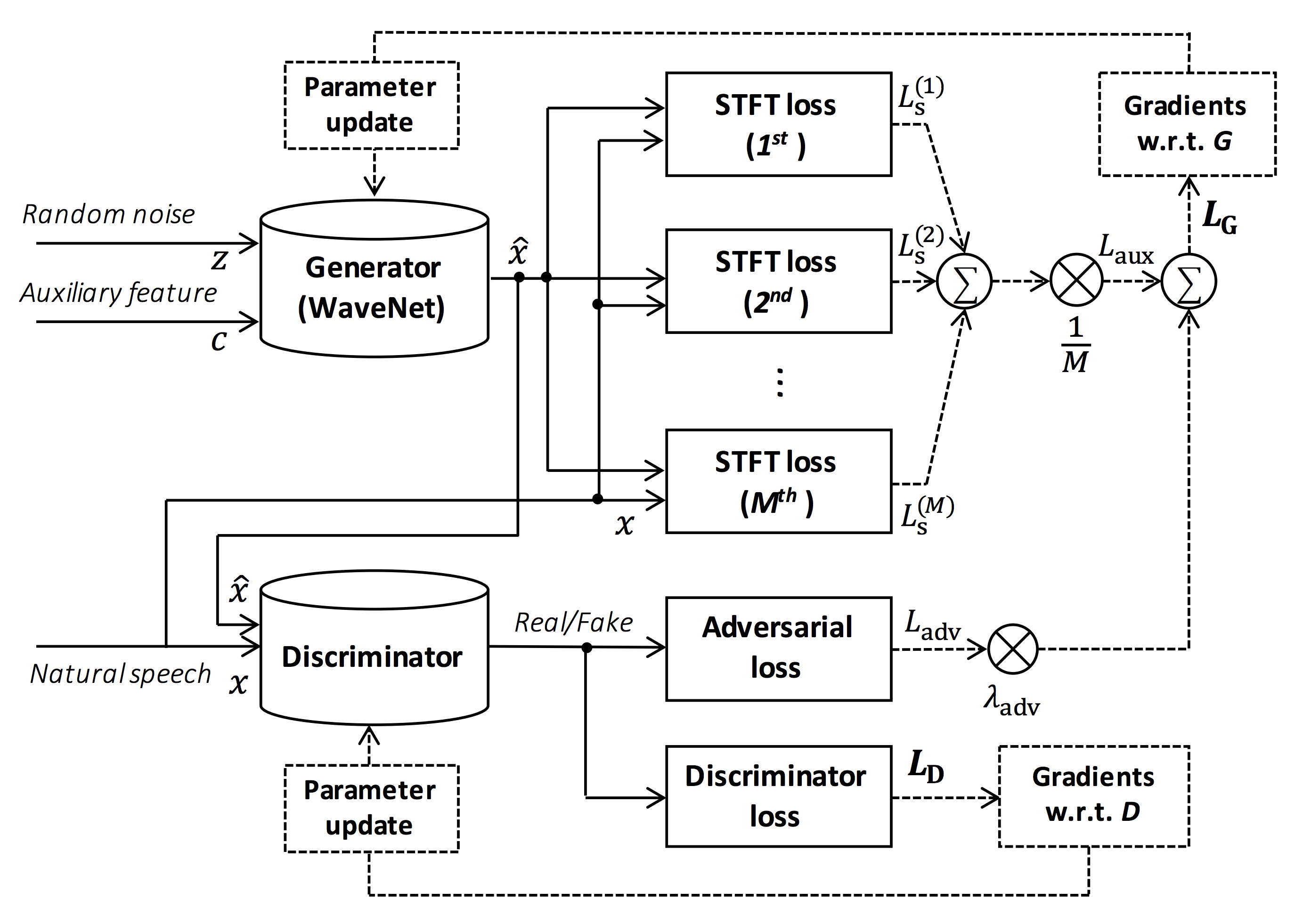
Source of the figure: https://arxiv.org/pdf/1910.11480.pdf

The goal of this repository is to provide real-time neural vocoder, which is compatible with ESPnet-TTS.
Also, this repository can be combined with NVIDIA/tacotron2-based implementation (See this comment).

You can try the real-time end-to-end text-to-speech and singing voice synthesis demonstration in Google Colab!

Real-time demonstration with ESPnet2
Real-time demonstration with ESPnet1
Real-time demonstration with Muskits

What's new

2023/08/17 LibriTTS-R recipe is available!
2022/02/27 Support singing voice vocoder [egs/{kiritan, opencpop, oniku_kurumi_utagoe_db, ofuton_p_utagoe_db, csd, kising}/voc1]
2021/10/21 Single-speaker Korean recipe [egs/kss/voc1] is available.
2021/08/24 Add more pretrained models of StyleMelGAN and HiFi-GAN.
2021/08/07 Add initial pretrained models of StyleMelGAN and HiFi-GAN.
2021/08/03 Support StyleMelGAN generator and discriminator!
2021/08/02 Support HiFi-GAN generator and discriminator!
2020/10/07 JSSS recipe is available!
2020/08/19 Real-time demo with ESPnet2 is available!
2020/05/29 VCTK, JSUT, and CSMSC multi-band MelGAN pretrained model is available!
2020/05/27 New LJSpeech multi-band MelGAN pretrained model is available!
2020/05/24 LJSpeech full-band MelGAN pretrained model is available!
2020/05/22 LJSpeech multi-band MelGAN pretrained model is available!
2020/05/16 Multi-band MelGAN is available!
2020/03/25 LibriTTS pretrained models are available!
2020/03/17 Tensorflow conversion example notebook is available (Thanks, @dathudeptrai)!
2020/03/16 LibriTTS recipe is available!
2020/03/12 PWG G + MelGAN D + STFT-loss samples are available!
2020/03/12 Multi-speaker English recipe egs/vctk/voc1 is available!
2020/02/22 MelGAN G + MelGAN D + STFT-loss samples are available!
2020/02/12 Support MelGAN's discriminator!
2020/02/08 Support MelGAN's generator!

Requirements

This repository is tested on Ubuntu 20.04 with a GPU Titan V.

Python 3.8+
Cuda 11.0+
CuDNN 8+
NCCL 2+ (for distributed multi-gpu training)
libsndfile (you can install via sudo apt install libsndfile-dev in ubuntu)
jq (you can install via sudo apt install jq in ubuntu)
sox (you can install via sudo apt install sox in ubuntu)

Different cuda version should be working but not explicitly tested.
All of the codes are tested on Pytorch 1.8.1, 1.9, 1.10.2, 1.11.0, 1.12.1, 1.13.1, 2.0.1 and 2.1.0.

Setup

You can select the installation method from two alternatives.

A. Use pip

$ git clone https://github.com/kan-bayashi/ParallelWaveGAN.git
$ cd ParallelWaveGAN
$ pip install -e .
# If you want to use distributed training, please install
# apex manually by following https://github.com/NVIDIA/apex
$ ...

Note that your cuda version must be exactly matched with the version used for the pytorch binary to install apex.
To install pytorch compiled with different cuda version, see tools/Makefile.

B. Make virtualenv

$ git clone https://github.com/kan-bayashi/ParallelWaveGAN.git
$ cd ParallelWaveGAN/tools
$ make
# If you want to use distributed training, please run following
# command to install apex.
$ make apex

Note that we specify cuda version used to compile pytorch wheel.
If you want to use different cuda version, please check tools/Makefile to change the pytorch wheel to be installed.

Recipe

This repository provides Kaldi-style recipes, as the same as ESPnet.
Currently, the following recipes are supported.

LJSpeech: English female speaker
JSUT: Japanese female speaker
JSSS: Japanese female speaker
CSMSC: Mandarin female speaker
CMU Arctic: English speakers
JNAS: Japanese multi-speaker
VCTK: English multi-speaker
LibriTTS: English multi-speaker
LibriTTS-R: English multi-speaker enhanced by speech restoration.
YesNo: English speaker (For debugging)
KSS: Single Korean female speaker
Oniku_kurumi_utagoe_db/: Single Japanese female singer (singing voice)
Kiritan: Single Japanese male singer (singing voice)
Ofuton_p_utagoe_db: Single Japanese female singer (singing voice)
Opencpop: Single Mandarin female singer (singing voice)
CSD: Single Korean/English female singer (singing voice)
KiSing: Single Mandarin female singer (singing voice)

To run the recipe, please follow the below instruction.

# Let us move on the recipe directory
$ cd egs/ljspeech/voc1

# Run the recipe from scratch
$ ./run.sh

# You can change config via command line
$ ./run.sh --conf <your_customized_yaml_config>

# You can select the stage to start and stop
$ ./run.sh --stage 2 --stop_stage 2

# If you want to specify the gpu
$ CUDA_VISIBLE_DEVICES=1 ./run.sh --stage 2

# If you want to resume training from 10000 steps checkpoint
$ ./run.sh --stage 2 --resume <path>/<to>/checkpoint-10000steps.pkl

See more info about the recipes in this README.

Speed

The decoding speed is RTF = 0.016 with TITAN V, much faster than the real-time.

[decode]: 100%|ââââââââââ| 250/250 [00:30<00:00,  8.31it/s, RTF=0.0156]
2019-11-03 09:07:40,480 (decode:127) INFO: finished generation of 250 utterances (RTF = 0.016).

Even on the CPU (Intel(R) Xeon(R) Gold 6154 CPU @ 3.00GHz 16 threads), it can generate less than the real-time.

[decode]: 100%|ââââââââââ| 250/250 [22:16<00:00,  5.35s/it, RTF=0.841]
2019-11-06 09:04:56,697 (decode:129) INFO: finished generation of 250 utterances (RTF = 0.734).

If you use MelGAN's generator, the decoding speed will be further faster.

# On CPU (Intel(R) Xeon(R) Gold 6154 CPU @ 3.00GHz 16 threads)
[decode]: 100%|ââââââââââ| 250/250 [04:00<00:00,  1.04it/s, RTF=0.0882]
2020-02-08 10:45:14,111 (decode:142) INFO: Finished generation of 250 utterances (RTF = 0.137).

# On GPU (TITAN V)
[decode]: 100%|ââââââââââ| 250/250 [00:06<00:00, 36.38it/s, RTF=0.00189]
2020-02-08 05:44:42,231 (decode:142) INFO: Finished generation of 250 utterances (RTF = 0.002).

If you use Multi-band MelGAN's generator, the decoding speed will be much further faster.

# On CPU (Intel(R) Xeon(R) Gold 6154 CPU @ 3.00GHz 16 threads)
[decode]: 100%|ââââââââââ| 250/250 [01:47<00:00,  2.95it/s, RTF=0.048]
2020-05-22 15:37:19,771 (decode:151) INFO: Finished generation of 250 utterances (RTF = 0.059).

# On GPU (TITAN V)
[decode]: 100%|ââââââââââ| 250/250 [00:05<00:00, 43.67it/s, RTF=0.000928]
2020-05-22 15:35:13,302 (decode:151) INFO: Finished generation of 250 utterances (RTF = 0.001).

If you want to accelerate the inference more, it is worthwhile to try the conversion from pytorch to tensorflow.
The example of the conversion is available in the notebook (Provided by @dathudeptrai).

Results

Here the results are summarized in the table.
You can listen to the samples and download pretrained models from the link to our google drive.

Model	Conf	Lang	Fs [Hz]	Mel range [Hz]	FFT / Hop / Win [pt]	# iters
ljspeech_parallel_wavegan.v1	link	EN	22.05k	80-7600	1024 / 256 / None	400k
ljspeech_parallel_wavegan.v1.long	link	EN	22.05k	80-7600	1024 / 256 / None	1M
ljspeech_parallel_wavegan.v1.no_limit	link	EN	22.05k	None	1024 / 256 / None	400k
ljspeech_parallel_wavegan.v3	link	EN	22.05k	80-7600	1024 / 256 / None	3M
ljspeech_melgan.v1	link	EN	22.05k	80-7600	1024 / 256 / None	400k
ljspeech_melgan.v1.long	link	EN	22.05k	80-7600	1024 / 256 / None	1M
ljspeech_melgan_large.v1	link	EN	22.05k	80-7600	1024 / 256 / None	400k
ljspeech_melgan_large.v1.long	link	EN	22.05k	80-7600	1024 / 256 / None	1M
ljspeech_melgan.v3	link	EN	22.05k	80-7600	1024 / 256 / None	2M
ljspeech_melgan.v3.long	link	EN	22.05k	80-7600	1024 / 256 / None	4M
ljspeech_full_band_melgan.v1	link	EN	22.05k	80-7600	1024 / 256 / None	1M
ljspeech_full_band_melgan.v2	link	EN	22.05k	80-7600	1024 / 256 / None	1M
ljspeech_multi_band_melgan.v1	link	EN	22.05k	80-7600	1024 / 256 / None	1M
ljspeech_multi_band_melgan.v2	link	EN	22.05k	80-7600	1024 / 256 / None	1M
ljspeech_hifigan.v1	link	EN	22.05k	80-7600	1024 / 256 / None	2.5M
ljspeech_style_melgan.v1	link	EN	22.05k	80-7600	1024 / 256 / None	1.5M
jsut_parallel_wavegan.v1	link	JP	24k	80-7600	2048 / 300 / 1200	400k
jsut_multi_band_melgan.v2	link	JP	24k	80-7600	2048 / 300 / 1200	1M
just_hifigan.v1	link	JP	24k	80-7600	2048 / 300 / 1200	2.5M
just_style_melgan.v1	link	JP	24k	80-7600	2048 / 300 / 1200	1.5M
csmsc_parallel_wavegan.v1	link	ZH	24k	80-7600	2048 / 300 / 1200	400k
csmsc_multi_band_melgan.v2	link	ZH	24k	80-7600	2048 / 300 / 1200	1M
csmsc_hifigan.v1	link	ZH	24k	80-7600	2048 / 300 / 1200	2.5M
csmsc_style_melgan.v1	link	ZH	24k	80-7600	2048 / 300 / 1200	1.5M
arctic_slt_parallel_wavegan.v1	link	EN	16k	80-7600	1024 / 256 / None	400k
jnas_parallel_wavegan.v1	link	JP	16k	80-7600	1024 / 256 / None	400k
vctk_parallel_wavegan.v1	link	EN	24k	80-7600	2048 / 300 / 1200	400k
vctk_parallel_wavegan.v1.long	link	EN	24k	80-7600	2048 / 300 / 1200	1M
vctk_multi_band_melgan.v2	link	EN	24k	80-7600	2048 / 300 / 1200	1M
vctk_hifigan.v1	link	EN	24k	80-7600	2048 / 300 / 1200	2.5M
vctk_style_melgan.v1	link	EN	24k	80-7600	2048 / 300 / 1200	1.5M
libritts_parallel_wavegan.v1	link	EN	24k	80-7600	2048 / 300 / 1200	400k
libritts_parallel_wavegan.v1.long	link	EN	24k	80-7600	2048 / 300 / 1200	1M
libritts_multi_band_melgan.v2	link	EN	24k	80-7600	2048 / 300 / 1200	1M
libritts_hifigan.v1	link	EN	24k	80-7600	2048 / 300 / 1200	2.5M
libritts_style_melgan.v1	link	EN	24k	80-7600	2048 / 300 / 1200	1.5M
kss_parallel_wavegan.v1	link	KO	24k	80-7600	2048 / 300 / 1200	400k
hui_acg_hokuspokus_parallel_wavegan.v1	link	DE	24k	80-7600	2048 / 300 / 1200	400k
ruslan_parallel_wavegan.v1	link	RU	24k	80-7600	2048 / 300 / 1200	400k
oniku_hifigan.v1	link	JP	24k	80-7600	2048 / 300 / 1200	250k
kiritan_hifigan.v1	link	JP	24k	80-7600	2048 / 300 / 1200	300k
ofuton_hifigan.v1	link	JP	24k	80-7600	2048 / 300 / 1200	300k
opencpop_hifigan.v1	link	ZH	24k	80-7600	2048 / 300 / 1200	250k
csd_english_hifigan.v1	link	EN	24k	80-7600	2048 / 300 / 1200	300k
csd_korean_hifigan.v1	link	EN	24k	80-7600	2048 / 300 / 1200	250k
kising_hifigan.v1	link	ZH	24k	80-7600	2048 / 300 / 1200	300k
m4singer_hifigan.v1	link	ZH	24k	80-7600	2048 / 300 / 1200	1M

Please access at our google drive to check more results.

Please check the license of database (e.g., whether it is proper for commercial usage) before using the pre-trained model.
The authors will not be responsible for any loss due to the use of the model and legal disputes regarding the use of the dataset.

How-to-use pretrained models

Analysis-synthesis

Here the minimal code is shown to perform analysis-synthesis using the pretrained model.

# Please make sure you installed `parallel_wavegan`
# If not, please install via pip
$ pip install parallel_wavegan

# You can download the pretrained model from terminal
$ python << EOF
from parallel_wavegan.utils import download_pretrained_model
download_pretrained_model("<pretrained_model_tag>", "pretrained_model")
EOF

# You can get all of available pretrained models as follows:
$ python << EOF
from parallel_wavegan.utils import PRETRAINED_MODEL_LIST
print(PRETRAINED_MODEL_LIST.keys())
EOF

# Now you can find downloaded pretrained model in `pretrained_model/<pretrain_model_tag>/`
$ ls pretrain_model/<pretrain_model_tag>
ï  checkpoint-400000steps.pkl  ï  config.yml  ï  stats.h5

# These files can also be downloaded manually from the above results

# Please put an audio file in `sample` directory to perform analysis-synthesis
$ ls sample/
ï  sample.wav

# Then perform feature extraction -> feature normalization -> synthesis
$ parallel-wavegan-preprocess \
    --config pretrain_model/<pretrain_model_tag>/config.yml \
    --rootdir sample \
    --dumpdir dump/sample/raw
100%|ââââââââââââââââââââââââââââââââââââââââ| 1/1 [00:00<00:00, 914.19it/s]
$ parallel-wavegan-normalize \
    --config pretrain_model/<pretrain_model_tag>/config.yml \
    --rootdir dump/sample/raw \
    --dumpdir dump/sample/norm \
    --stats pretrain_model/<pretrain_model_tag>/stats.h5
2019-11-13 13:44:29,574 (normalize:87) INFO: the number of files = 1.
100%|ââââââââââââââââââââââââââââââââââââââââ| 1/1 [00:00<00:00, 513.13it/s]
$ parallel-wavegan-decode \
    --checkpoint pretrain_model/<pretrain_model_tag>/checkpoint-400000steps.pkl \
    --dumpdir dump/sample/norm \
    --outdir sample
2019-11-13 13:44:31,229 (decode:91) INFO: the number of features to be decoded = 1.
[decode]: 100%|âââââââââââââââââââ| 1/1 [00:00<00:00, 18.33it/s, RTF=0.0146]
2019-11-13 13:44:37,132 (decode:129) INFO: finished generation of 1 utterances (RTF = 0.015).

# You can skip normalization step (on-the-fly normalization, feature extraction -> synthesis)
$ parallel-wavegan-preprocess \
    --config pretrain_model/<pretrain_model_tag>/config.yml \
    --rootdir sample \
    --dumpdir dump/sample/raw
100%|ââââââââââââââââââââââââââââââââââââââââ| 1/1 [00:00<00:00, 914.19it/s]
$ parallel-wavegan-decode \
    --checkpoint pretrain_model/<pretrain_model_tag>/checkpoint-400000steps.pkl \
    --dumpdir dump/sample/raw \
    --normalize-before \
    --outdir sample
2019-11-13 13:44:31,229 (decode:91) INFO: the number of features to be decoded = 1.
[decode]: 100%|âââââââââââââââââââ| 1/1 [00:00<00:00, 18.33it/s, RTF=0.0146]
2019-11-13 13:44:37,132 (decode:129) INFO: finished generation of 1 utterances (RTF = 0.015).

# you can find the generated speech in `sample` directory
$ ls sample
ï  sample.wav  ï  sample_gen.wav

Decoding with ESPnet-TTS model's features

Here, I show the procedure to generate waveforms with features generated by ESPnet-TTS models.

# Make sure you already finished running the recipe of ESPnet-TTS.
# You must use the same feature settings for both Text2Mel and Mel2Wav models.
# Let us move on "ESPnet" recipe directory
$ cd /path/to/espnet/egs/<recipe_name>/tts1
$ pwd
/path/to/espnet/egs/<recipe_name>/tts1

# If you use ESPnet2, move on `egs2/`
$ cd /path/to/espnet/egs2/<recipe_name>/tts1
$ pwd
/path/to/espnet/egs2/<recipe_name>/tts1

# Please install this repository in ESPnet conda (or virtualenv) environment
$ . ./path.sh && pip install -U parallel_wavegan

# You can download the pretrained model from terminal
$ python << EOF
from parallel_wavegan.utils import download_pretrained_model
download_pretrained_model("<pretrained_model_tag>", "pretrained_model")
EOF

# You can get all of available pretrained models as follows:
$ python << EOF
from parallel_wavegan.utils import PRETRAINED_MODEL_LIST
print(PRETRAINED_MODEL_LIST.keys())
EOF

# You can find downloaded pretrained model in `pretrained_model/<pretrain_model_tag>/`
$ ls pretrain_model/<pretrain_model_tag>
ï  checkpoint-400000steps.pkl  ï  config.yml  ï  stats.h5

# These files can also be downloaded manually from the above results

Case 1: If you use the same dataset for both Text2Mel and Mel2Wav

# In this case, you can directly use generated features for decoding.
# Please specify `feats.scp` path for `--feats-scp`, which is located in
# exp/<your_model_dir>/outputs_*_decode/<set_name>/feats.scp.
# Note that do not use outputs_*decode_denorm/<set_name>/feats.scp since
# it is de-normalized features (the input for PWG is normalized features).
$ parallel-wavegan-decode \
    --checkpoint pretrain_model/<pretrain_model_tag>/checkpoint-400000steps.pkl \
    --feats-scp exp/<your_model_dir>/outputs_*_decode/<set_name>/feats.scp \
    --outdir <path_to_outdir>

# In the case of ESPnet2, the generated feature can be found in
# exp/<your_model_dir>/decode_*/<set_name>/norm/feats.scp.
$ parallel-wavegan-decode \
    --checkpoint pretrain_model/<pretrain_model_tag>/checkpoint-400000steps.pkl \
    --feats-scp exp/<your_model_dir>/decode_*/<set_name>/norm/feats.scp \
    --outdir <path_to_outdir>

# You can find the generated waveforms in <path_to_outdir>/.
$ ls <path_to_outdir>
ï  utt_id_1_gen.wav  ï  utt_id_2_gen.wav  ...  ï  utt_id_N_gen.wav

Case 2: If you use different datasets for Text2Mel and Mel2Wav models

# In this case, you must provide `--normalize-before` option additionally.
# And use `feats.scp` of de-normalized generated features.

# ESPnet1 case
$ parallel-wavegan-decode \
    --checkpoint pretrain_model/<pretrain_model_tag>/checkpoint-400000steps.pkl \
    --feats-scp exp/<your_model_dir>/outputs_*_decode_denorm/<set_name>/feats.scp \
    --outdir <path_to_outdir> \
    --normalize-before

# ESPnet2 case
$ parallel-wavegan-decode \
    --checkpoint pretrain_model/<pretrain_model_tag>/checkpoint-400000steps.pkl \
    --feats-scp exp/<your_model_dir>/decode_*/<set_name>/denorm/feats.scp \
    --outdir <path_to_outdir> \
    --normalize-before

# You can find the generated waveforms in <path_to_outdir>/.
$ ls <path_to_outdir>
ï  utt_id_1_gen.wav  ï  utt_id_2_gen.wav  ...  ï  utt_id_N_gen.wav

If you want to combine these models in python, you can try the real-time demonstration in Google Colab!

Real-time demonstration with ESPnet2
Real-time demonstration with ESPnet1

Decoding with dumped npy files

Sometimes we want to decode with dumped npy files, which are mel-spectrogram generated by TTS models. Please make sure you used the same feature extraction settings of the pretrained vocoder (fs, fft_size, hop_size, win_length, fmin, and fmax).
Only the difference of log_base can be changed with some post-processings (we use log 10 instead of natural log as a default). See detail in the comment.

# Generate dummy npy file of mel-spectrogram
$ ipython
[ins] In [1]: import numpy as np
[ins] In [2]: x = np.random.randn(512, 80)  # (#frames, #mels)
[ins] In [3]: np.save("dummy_1.npy", x)
[ins] In [4]: y = np.random.randn(256, 80)  # (#frames, #mels)
[ins] In [5]: np.save("dummy_2.npy", y)
[ins] In [6]: exit

# Make scp file (key-path format)
$ find -name "*.npy" | awk '{print "dummy_" NR " " $1}' > feats.scp

# Check (<utt_id> <path>)
$ cat feats.scp
dummy_1 ./dummy_1.npy
dummy_2 ./dummy_2.npy

# Decode without feature normalization
# This case assumes that the input mel-spectrogram is normalized with the same statistics of the pretrained model.
$ parallel-wavegan-decode \
    --checkpoint /path/to/checkpoint-400000steps.pkl \
    --feats-scp ./feats.scp \
    --outdir wav
2021-08-10 09:13:07,624 (decode:140) INFO: The number of features to be decoded = 2.
[decode]: 100%|ââââââââââââââââââââââââââââââââââââââââ| 2/2 [00:00<00:00, 13.84it/s, RTF=0.00264]
2021-08-10 09:13:29,660 (decode:174) INFO: Finished generation of 2 utterances (RTF = 0.005).

# Decode with feature normalization
# This case assumes that the input mel-spectrogram is not normalized.
$ parallel-wavegan-decode \
    --checkpoint /path/to/checkpoint-400000steps.pkl \
    --feats-scp ./feats.scp \
    --normalize-before \
    --outdir wav
2021-08-10 09:13:07,624 (decode:140) INFO: The number of features to be decoded = 2.
[decode]: 100%|ââââââââââââââââââââââââââââââââââââââââ| 2/2 [00:00<00:00, 13.84it/s, RTF=0.00264]
2021-08-10 09:13:29,660 (decode:174) INFO: Finished generation of 2 utterances (RTF = 0.005).

Notes

The terms of use of the pretrained model follow that of each corpus used for the training. Please carefully check by yourself.
Some codes are derived from ESPnet or Kaldi, which are based on Apache-2.0 licenese.

References

Acknowledgement

The author would like to thank Ryuichi Yamamoto (@r9y9) for his great repository, paper, and valuable discussions.

Author

Tomoki Hayashi (@kan-bayashi)
E-mail: hayashi.tomoki<at>g.sp.m.is.nagoya-u.ac.jp

Top Related Projects

Convert designs to code with AI

Introducing Visual Copilot: A new AI model to turn Figma designs to high quality code using your components.

Try Visual Copilot