 BayesianOptimization
A Python implementation of global optimization with gaussian processes.
Top Related Projects
A Python implementation of global optimization with gaussian processes.

Distributed Asynchronous Hyperparameter Optimization in Python

Sequential model-based optimization with a `scipy.optimize` interface

Adaptive Experimentation Platform

A hyperparameter optimization framework

A fast library for AutoML and tuning. Join our Discord: https://discord.gg/Cppx2vSPVP.
Quick Overview
BayesianOptimization is a Python library for global optimization of black-box functions using Bayesian optimization techniques. It provides a flexible and efficient implementation of Gaussian Process-based optimization, suitable for various applications including hyperparameter tuning, experimental design, and function optimization.
Pros
- Easy to use and integrate with existing Python projects
- Supports both synchronous and asynchronous optimization
- Highly customizable with various acquisition functions and GP kernels
- Efficient for optimizing expensive-to-evaluate functions
Cons
- Limited to continuous parameter spaces
- May struggle with high-dimensional problems (>20 dimensions)
- Requires some understanding of Bayesian optimization concepts for optimal use
- Documentation could be more comprehensive for advanced features
Code Examples
- Basic usage:
from bayes_opt import BayesianOptimization

def black_box_function(x, y):
    return -x**2 - (y-1)**2 + 1

pbounds = {'x': (-2, 2), 'y': (-3, 3)}

optimizer = BayesianOptimization(
    f=black_box_function,
    pbounds=pbounds,
    random_state=1,
)

optimizer.maximize(
    init_points=2,
    n_iter=3,
)
- Using a custom acquisition function:
from bayes_opt import BayesianOptimization
from bayes_opt.util import UtilityFunction

def custom_acq(x, model):
    return -model.predict(x)[0]

utility = UtilityFunction(kind="custom", kappa=2.5, kappa_decay=0.5, custom_acq=custom_acq)

optimizer = BayesianOptimization(
    f=black_box_function,
    pbounds=pbounds,
)

optimizer.maximize(
    init_points=2,
    n_iter=3,
    acquisition_function=utility
)
- Asynchronous optimization:
from bayes_opt import AsyncBayesianOptimization

optimizer = AsyncBayesianOptimization(
    f=black_box_function,
    pbounds=pbounds,
)

for _ in range(10):
    optimizer.maximize(init_points=1, n_iter=1)
    # Simulate asynchronous evaluation
    optimizer.set_pump_function(lambda x: black_box_function(**x))
Getting Started
To get started with BayesianOptimization:
-
Install the library:
pip install bayesian-optimization -
Import and use in your Python script:
from bayes_opt import BayesianOptimization

def your_objective_function(x, y):
    return x**2 + y**2

pbounds = {'x': (-5, 5), 'y': (-5, 5)}

optimizer = BayesianOptimization(
    f=your_objective_function,
    pbounds=pbounds,
    random_state=1,
)

optimizer.maximize(
    init_points=5,
    n_iter=10,
)

print(optimizer.max)
This will set up a basic optimization process for your objective function within the specified parameter bounds.
Competitor Comparisons
A Python implementation of global optimization with gaussian processes.
Pros of BayesianOptimization
- Well-established and widely used library for Bayesian optimization
- Extensive documentation and examples available
- Supports various acquisition functions and GP kernels
Cons of BayesianOptimization
- Limited support for categorical variables
- May require more manual tuning compared to some alternatives
- Lacks built-in parallelization capabilities
Code Comparison
BayesianOptimization:
from bayes_opt import BayesianOptimization

def black_box_function(x, y):
    return -x**2 - (y-1)**2 + 1

pbounds = {'x': (-2, 2), 'y': (-3, 3)}

optimizer = BayesianOptimization(
    f=black_box_function,
    pbounds=pbounds,
    random_state=1,
)

optimizer.maximize(
    init_points=2,
    n_iter=3,
)
Note: The code comparison is not applicable in this case as we are comparing the same repository to itself. The provided code snippet demonstrates the basic usage of BayesianOptimization.
Distributed Asynchronous Hyperparameter Optimization in Python
Pros of Hyperopt
- More flexible search space definition, allowing for conditional and nested parameters
- Supports multiple optimization algorithms (TPE, random search, adaptive TPE)
- Includes built-in parallel optimization capabilities
Cons of Hyperopt
- Steeper learning curve due to more complex API
- Less focused on Bayesian optimization specifically
- May be overkill for simpler optimization tasks
Code Comparison
BayesianOptimization:
from bayes_opt import BayesianOptimization

pbounds = {'x': (2, 4), 'y': (-3, 3)}
optimizer = BayesianOptimization(f=black_box_function, pbounds=pbounds)
optimizer.maximize(init_points=2, n_iter=3)
Hyperopt:
from hyperopt import fmin, tpe, hp

space = {'x': hp.uniform('x', 2, 4), 'y': hp.uniform('y', -3, 3)}
best = fmin(fn=objective, space=space, algo=tpe.suggest, max_evals=5)
Both libraries offer powerful optimization capabilities, but Hyperopt provides more flexibility and advanced features at the cost of increased complexity. BayesianOptimization is more straightforward and focused on Bayesian optimization specifically, making it easier to use for simpler tasks. The choice between the two depends on the specific requirements of your optimization problem and your familiarity with the libraries.
Sequential model-based optimization with a `scipy.optimize` interface
Pros of scikit-optimize
- Broader range of optimization algorithms, including gradient-based methods
- Integrated with scikit-learn, allowing easy use with machine learning workflows
- More extensive documentation and examples
Cons of scikit-optimize
- Slightly more complex API, which may be less intuitive for beginners
- Slower performance for some use cases compared to BayesianOptimization
Code Comparison
BayesianOptimization:
from bayes_opt import BayesianOptimization

optimizer = BayesianOptimization(
    f=black_box_function,
    pbounds={'x': (-2, 2), 'y': (-3, 3)},
    random_state=1,
)
optimizer.maximize(init_points=2, n_iter=3)
scikit-optimize:
from skopt import gp_minimize

res = gp_minimize(
    func=black_box_function,
    dimensions=[(-2.0, 2.0), (-3.0, 3.0)],
    n_calls=5,
    random_state=1,
)
Both libraries offer Bayesian optimization capabilities, but scikit-optimize provides a wider range of algorithms and integrates well with the scikit-learn ecosystem. BayesianOptimization, on the other hand, offers a simpler API and may be faster for certain applications. The choice between the two depends on the specific requirements of your project and your familiarity with the libraries.
Adaptive Experimentation Platform
Pros of Ax
- More comprehensive framework for adaptive experimentation
- Supports multi-objective optimization and constrained optimization
- Integrates with PyTorch for machine learning experiments
Cons of Ax
- Steeper learning curve due to more complex API
- Heavier dependencies and larger codebase
- May be overkill for simpler optimization tasks
Code Comparison
BayesianOptimization:
from bayes_opt import BayesianOptimization

def black_box_function(x, y):
    return -x ** 2 - (y - 1) ** 2 + 1

optimizer = BayesianOptimization(
    f=black_box_function,
    pbounds={'x': (-2, 2), 'y': (-3, 3)},
    random_state=1,
)

optimizer.maximize(init_points=2, n_iter=3)
Ax:
from ax import optimize

def evaluation_function(parameters):
    x, y = parameters["x"], parameters["y"]
    return -x ** 2 - (y - 1) ** 2 + 1

best_parameters, values, experiment, model = optimize(
    parameters=[
        {"name": "x", "type": "range", "bounds": [-2.0, 2.0]},
        {"name": "y", "type": "range", "bounds": [-3.0, 3.0]},
    ],
    evaluation_function=evaluation_function,
    objective_name="score",
    total_trials=5,
)
A hyperparameter optimization framework
Pros of Optuna
- More comprehensive and feature-rich, supporting various optimization algorithms beyond Bayesian optimization
- Better suited for large-scale hyperparameter optimization tasks with distributed computing capabilities
- Offers a user-friendly interface with visualization tools and integration with popular ML frameworks
Cons of Optuna
- May have a steeper learning curve due to its more extensive feature set
- Potentially overkill for simpler optimization tasks where BayesianOptimization might suffice
Code Comparison
Optuna:
import optuna

def objective(trial):
    x = trial.suggest_float('x', -10, 10)
    return (x - 2) ** 2

study = optuna.create_study()
study.optimize(objective, n_trials=100)
BayesianOptimization:
from bayes_opt import BayesianOptimization

def objective(x):
    return -(x - 2) ** 2

optimizer = BayesianOptimization(f=objective, pbounds={'x': (-10, 10)})
optimizer.maximize(init_points=2, n_iter=98)
Both libraries provide straightforward ways to define and optimize objective functions, but Optuna's interface is more flexible and allows for easier integration with complex ML workflows.
A fast library for AutoML and tuning. Join our Discord: https://discord.gg/Cppx2vSPVP.
Pros of FLAML
- Broader scope: Supports automated machine learning (AutoML) and hyperparameter tuning for various ML tasks
- More efficient: Uses cost-aware search strategies for faster optimization
- Easier integration: Provides high-level APIs for common ML frameworks and tasks
Cons of FLAML
- Steeper learning curve: More complex due to its broader functionality
- Less flexibility: May be overkill for simple Bayesian optimization tasks
- Heavier dependencies: Requires more external libraries
Code Comparison
FLAML:
from flaml import AutoML
automl = AutoML()
automl.fit(X_train, y_train, task="classification")
predictions = automl.predict(X_test)
BayesianOptimization:
from bayes_opt import BayesianOptimization
optimizer = BayesianOptimization(f=black_box_function, pbounds=parameter_bounds)
optimizer.maximize(init_points=5, n_iter=20)
Summary
FLAML offers a more comprehensive AutoML solution with efficient search strategies, while BayesianOptimization provides a focused tool for Bayesian optimization tasks. FLAML is better suited for complex ML workflows, while BayesianOptimization excels in simpler optimization scenarios. The choice between the two depends on the specific requirements of your project and the level of control you need over the optimization process.
Convert  designs to code with AI

Introducing Visual Copilot: A new AI model to turn Figma designs to high quality code using your components.
Try Visual CopilotREADME
Bayesian Optimization
![]()
![]()


Pure Python implementation of bayesian global optimization with gaussian processes.
This is a constrained global optimization package built upon bayesian inference and gaussian processes, that attempts to find the maximum value of an unknown function in as few iterations as possible. This technique is particularly suited for optimization of high cost functions and situations where the balance between exploration and exploitation is important.
Installation
- pip (via PyPI):
$ pip install bayesian-optimization
- Conda (via conda-forge):
$ conda install -c conda-forge bayesian-optimization
How does it work?
See the documentation for how to use this package.
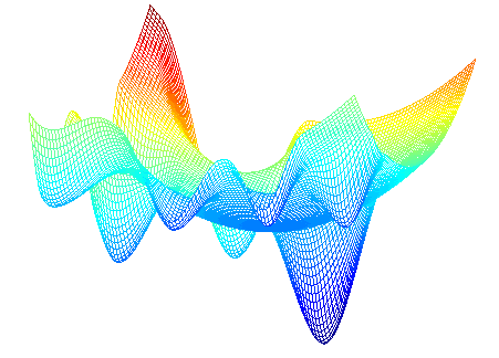
Bayesian optimization works by constructing a posterior distribution of functions (gaussian process) that best describes the function you want to optimize. As the number of observations grows, the posterior distribution improves, and the algorithm becomes more certain of which regions in parameter space are worth exploring and which are not, as seen in the picture below.

As you iterate over and over, the algorithm balances its needs of exploration and exploitation taking into account what it knows about the target function. At each step a Gaussian Process is fitted to the known samples (points previously explored), and the posterior distribution, combined with a exploration strategy (such as UCB (Upper Confidence Bound), or EI (Expected Improvement)), are used to determine the next point that should be explored (see the gif below).

This process is designed to minimize the number of steps required to find a combination of parameters that are close to the optimal combination. To do so, this method uses a proxy optimization problem (finding the maximum of the acquisition function) that, albeit still a hard problem, is cheaper (in the computational sense) and common tools can be employed. Therefore Bayesian Optimization is most adequate for situations where sampling the function to be optimized is a very expensive endeavor. See the references for a proper discussion of this method.
This project is under active development. If you run into trouble, find a bug or notice anything that needs correction, please let us know by filing an issue.
Basic tour of the Bayesian Optimization package
1. Specifying the function to be optimized
This is a function optimization package, therefore the first and most important ingredient is, of course, the function to be optimized.
DISCLAIMER: We know exactly how the output of the function below depends on its parameter. Obviously this is just an example, and you shouldn't expect to know it in a real scenario. However, it should be clear that you don't need to. All you need in order to use this package (and more generally, this technique) is a function f that takes a known set of parameters and outputs a real number.
def black_box_function(x, y):
    """Function with unknown internals we wish to maximize.

    This is just serving as an example, for all intents and
    purposes think of the internals of this function, i.e.: the process
    which generates its output values, as unknown.
    """
    return -x ** 2 - (y - 1) ** 2 + 1
2. Getting Started
All we need to get started is to instantiate a BayesianOptimization object specifying a function to be optimized f, and its parameters with their corresponding bounds, pbounds. This is a constrained optimization technique, so you must specify the minimum and maximum values that can be probed for each parameter in order for it to work
from bayes_opt import BayesianOptimization

# Bounded region of parameter space
pbounds = {'x': (2, 4), 'y': (-3, 3)}

optimizer = BayesianOptimization(
    f=black_box_function,
    pbounds=pbounds,
    random_state=1,
)
The BayesianOptimization object will work out of the box without much tuning needed. The main method you should be aware of is maximize, which does exactly what you think it does.
There are many parameters you can pass to maximize, nonetheless, the most important ones are:
n_iter: How many steps of bayesian optimization you want to perform. The more steps the more likely to find a good maximum you are.init_points: How many steps of random exploration you want to perform. Random exploration can help by diversifying the exploration space.
optimizer.maximize(
    init_points=2,
    n_iter=3,
)
|   iter    |  target   |     x     |     y     |
-------------------------------------------------
|  1        | -7.135    |  2.834    |  1.322    |
|  2        | -7.78     |  2.0      | -1.186    |
|  3        | -19.0     |  4.0      |  3.0      |
|  4        | -16.3     |  2.378    | -2.413    |
|  5        | -4.441    |  2.105    | -0.005822 |
=================================================
The best combination of parameters and target value found can be accessed via the property optimizer.max.
print(optimizer.max)
>>> {'target': -4.441293113411222, 'params': {'y': -0.005822117636089974, 'x': 2.104665051994087}}
While the list of all parameters probed and their corresponding target values is available via the property optimizer.res.
for i, res in enumerate(optimizer.res):
    print("Iteration {}: \n\t{}".format(i, res))

>>> Iteration 0:
>>>     {'target': -7.135455292718879, 'params': {'y': 1.3219469606529488, 'x': 2.8340440094051482}}
>>> Iteration 1:
>>>     {'target': -7.779531005607566, 'params': {'y': -1.1860045642089614, 'x': 2.0002287496346898}}
>>> Iteration 2:
>>>     {'target': -19.0, 'params': {'y': 3.0, 'x': 4.0}}
>>> Iteration 3:
>>>     {'target': -16.29839645063864, 'params': {'y': -2.412527795983739, 'x': 2.3776144540856503}}
>>> Iteration 4:
>>>     {'target': -4.441293113411222, 'params': {'y': -0.005822117636089974, 'x': 2.104665051994087}}
Minutiae
Citation
If you used this package in your research, please cite it:
@Misc{,
    author = {Fernando Nogueira},
    title = {{Bayesian Optimization}: Open source constrained global optimization tool for {Python}},
    year = {2014--},
    url = " https://github.com/bayesian-optimization/BayesianOptimization"
}
If you used any of the advanced functionalities, please additionally cite the corresponding publication:
For the SequentialDomainTransformer:
@article{
    author = {Stander, Nielen and Craig, Kenneth},
    year = {2002},
    month = {06},
    pages = {},
    title = {On the robustness of a simple domain reduction scheme for simulation-based optimization},
    volume = {19},
    journal = {International Journal for Computer-Aided Engineering and Software (Eng. Comput.)},
    doi = {10.1108/02644400210430190}
}
For constrained optimization:
@inproceedings{gardner2014bayesian,
    title={Bayesian optimization with inequality constraints.},
    author={Gardner, Jacob R and Kusner, Matt J and Xu, Zhixiang Eddie and Weinberger, Kilian Q and Cunningham, John P},
    booktitle={ICML},
    volume={2014},
    pages={937--945},
    year={2014}
}
For optimization over non-float parameters:
@article{garrido2020dealing,
  title={Dealing with categorical and integer-valued variables in bayesian optimization with gaussian processes},
  author={Garrido-Merch{\'a}n, Eduardo C and Hern{\'a}ndez-Lobato, Daniel},
  journal={Neurocomputing},
  volume={380},
  pages={20--35},
  year={2020},
  publisher={Elsevier}
}
Top Related Projects
A Python implementation of global optimization with gaussian processes.
Distributed Asynchronous Hyperparameter Optimization in Python
Sequential model-based optimization with a `scipy.optimize` interface
Adaptive Experimentation Platform
A hyperparameter optimization framework
A fast library for AutoML and tuning. Join our Discord: https://discord.gg/Cppx2vSPVP.
Convert designs to code with AI
Introducing Visual Copilot: A new AI model to turn Figma designs to high quality code using your components.
Try Visual Copilot