visdom

A flexible tool for creating, organizing, and sharing visualizations of live, rich data. Supports Torch and Numpy.

9,972

1,137

9,972

116

View on GitHub

Top Related Projects

dash

21,148

Data Apps & Dashboards for Python. No JavaScript Required.

holoviews

2,687

With Holoviews, your data visualizes itself.

wandb

8,869

The AI developer platform. Use Weights & Biases to train and fine-tune models, and manage models from experimentation to production.

mlflow

18,287

Open source platform for the machine learning lifecycle

Quick Overview

Visdom is a flexible tool for creating and organizing visualizations of live, rich data. It aims to facilitate rapid creation of visualizations for machine learning experiments, with support for various plot types and the ability to update plots in real-time.

Pros

Supports a wide range of visualization types, including plots, images, and text
Allows real-time updates of visualizations, ideal for monitoring ongoing experiments
Provides a web-based interface for easy access and sharing of visualizations
Integrates well with popular machine learning frameworks like PyTorch

Cons

Requires running a separate server process, which can be cumbersome for some users
Documentation can be sparse or outdated in some areas
May have performance issues with very large datasets or frequent updates
Less actively maintained compared to some other visualization libraries

Code Examples

Creating a simple line plot:

import visdom
import numpy as np

vis = visdom.Visdom()

Y = np.linspace(0, 10, 100)
X = np.sin(Y)

vis.line(X=Y, Y=X, opts=dict(title='Sine Wave', xlabel='X', ylabel='Y'))

Updating a plot in real-time:

import visdom
import numpy as np
import time

vis = visdom.Visdom()

plot = vis.line(Y=np.array([0]), opts=dict(title='Dynamic Plot'))

for i in range(100):
    time.sleep(0.1)
    vis.line(Y=np.array([i]), X=np.array([i]), win=plot, update='append')

Displaying an image:

import visdom
import numpy as np

vis = visdom.Visdom()

# Create a random 3-channel image
img = np.random.rand(3, 256, 256)

vis.image(img, opts=dict(title='Random Image', caption='A randomly generated image'))

Getting Started

To get started with Visdom:

Install Visdom:
```
pip install visdom
```
Start the Visdom server:
```
python -m visdom.server
```
In your Python script, import and initialize Visdom:
```
import visdom
vis = visdom.Visdom()
```
Create visualizations using the vis object, as shown in the code examples above.
Open a web browser and navigate to http://localhost:8097 to view your visualizations.

Competitor Comparisons

dash

21,148

Data Apps & Dashboards for Python. No JavaScript Required.

Pros of Dash

More comprehensive and feature-rich framework for building full-fledged web applications
Better documentation and larger community support
Seamless integration with Plotly's interactive plotting library

Cons of Dash

Steeper learning curve, especially for those new to web development
Requires more setup and boilerplate code compared to Visdom's simplicity
Can be overkill for simple visualization tasks

Code Comparison

Visdom:

import visdom
vis = visdom.Visdom()
vis.line(X=x, Y=y, win='line_plot', opts=dict(title='Simple Line Plot'))

Dash:

import dash
import dash_core_components as dcc
import dash_html_components as html
from dash.dependencies import Input, Output

app = dash.Dash(__name__)
app.layout = html.Div([
    dcc.Graph(id='line-plot', figure={'data': [{'x': x, 'y': y, 'type': 'line'}]})
])

Summary

Visdom is simpler and more lightweight, ideal for quick visualizations in machine learning workflows. Dash offers a more powerful framework for building interactive web applications with advanced features and customization options. Choose Visdom for rapid prototyping and simple plots, while Dash is better suited for creating complex, production-ready dashboards and applications.

holoviews

2,687

With Holoviews, your data visualizes itself.

Pros of HoloViews

More flexible and powerful data exploration capabilities
Seamless integration with Jupyter notebooks and other scientific Python libraries
Supports a wider range of plot types and customization options

Cons of HoloViews

Steeper learning curve due to its more complex API
May be overkill for simple visualization tasks
Requires more setup and configuration compared to Visdom

Code Comparison

HoloViews:

import holoviews as hv
import numpy as np

curve = hv.Curve(np.random.randn(100).cumsum())
hv.render(curve)

Visdom:

import visdom
import numpy as np

vis = visdom.Visdom()
Y = np.random.randn(100).cumsum()
vis.line(Y, opts=dict(title='Random Curve'))

Summary

HoloViews offers more advanced features and flexibility for data visualization, making it suitable for complex data exploration tasks. However, it may be more challenging to learn and set up compared to Visdom. Visdom provides a simpler interface for basic visualizations and real-time plotting, which can be advantageous for quick prototyping or monitoring tasks. The choice between the two depends on the specific requirements of your project and your familiarity with data visualization libraries.

wandb

8,869

The AI developer platform. Use Weights & Biases to train and fine-tune models, and manage models from experimentation to production.

Pros of wandb

More comprehensive experiment tracking and visualization capabilities
Integrates with popular ML frameworks like PyTorch and TensorFlow
Offers cloud-based collaboration and sharing features

Cons of wandb

Requires an account and potentially paid plans for advanced features
May have a steeper learning curve for beginners

Code comparison

wandb:

import wandb

wandb.init(project="my-project")
wandb.config.hyperparameters = {
    "learning_rate": 0.01,
    "epochs": 100
}
wandb.log({"accuracy": 0.9, "loss": 0.1})

visdom:

import visdom
import numpy as np

vis = visdom.Visdom()
vis.line(Y=np.random.rand(10), opts=dict(title='Test'))

Summary

wandb offers a more feature-rich and collaborative platform for experiment tracking and visualization, while visdom provides a simpler, lightweight solution for basic plotting needs. wandb's integration with popular ML frameworks and cloud-based features make it suitable for larger projects and teams, whereas visdom may be preferred for quick, local visualizations without the need for account setup or potential costs.

tensorboard

6,659

TensorFlow's Visualization Toolkit

Pros of TensorBoard

More comprehensive and feature-rich visualization tool
Tightly integrated with TensorFlow ecosystem
Supports distributed training and multi-worker setups

Cons of TensorBoard

Steeper learning curve for beginners
Primarily designed for TensorFlow, less flexible for other frameworks
Can be resource-intensive for large-scale experiments

Code Comparison

TensorBoard:

import tensorflow as tf

writer = tf.summary.create_file_writer("logs/")
with writer.as_default():
    tf.summary.scalar("loss", 0.1, step=1)

Visdom:

import visdom
import numpy as np

vis = visdom.Visdom()
vis.line(Y=np.array([0.1]), X=np.array([1]), win='loss', opts=dict(title='Loss'))

Key Differences

TensorBoard offers a more extensive set of visualization options
Visdom provides a simpler, more lightweight interface
TensorBoard is deeply integrated with TensorFlow, while Visdom is framework-agnostic
Visdom allows for real-time updates, whereas TensorBoard typically works with logged data
TensorBoard has better support for large-scale experiments and distributed training

Both tools serve similar purposes but cater to different use cases and preferences. TensorBoard is more suitable for complex TensorFlow projects, while Visdom offers a flexible solution for quick visualizations across various frameworks.

mlflow

18,287

Open source platform for the machine learning lifecycle

Pros of MLflow

More comprehensive ML lifecycle management, including experiment tracking, model packaging, and deployment
Better integration with popular ML frameworks and cloud platforms
Active development and larger community support

Cons of MLflow

Steeper learning curve due to more extensive features
Requires more setup and configuration for full functionality

Code Comparison

MLflow:

import mlflow

mlflow.start_run()
mlflow.log_param("param1", 5)
mlflow.log_metric("accuracy", 0.85)
mlflow.end_run()

Visdom:

from visdom import Visdom

viz = Visdom()
viz.line([0.5, 0.7, 0.9], [1, 2, 3], opts=dict(title='Test'))

Summary

MLflow offers a more comprehensive solution for ML lifecycle management, while Visdom focuses primarily on visualization. MLflow provides better integration with ML frameworks and cloud platforms, but has a steeper learning curve. Visdom is simpler to set up and use for basic visualization tasks, but lacks the extensive features of MLflow for experiment tracking and model management. The code examples demonstrate MLflow's focus on logging parameters and metrics, while Visdom emphasizes creating visualizations directly.

Convert designs to code with AI

Introducing Visual Copilot: A new AI model to turn Figma designs to high quality code using your components.

Try Visual Copilot

README

Creating, organizing & sharing visualizations of live, rich data. Supports Python.

Jump To: Setup, Usage, API, Customizing, Contributing, License

Visdom aims to facilitate visualization of (remote) data with an emphasis on supporting scientific experimentation.
Broadcast visualizations of plots, images, and text for yourself and your collaborators. Organize your visualization space programmatically or through the UI to create dashboards for live data, inspect results of experiments, or debug experimental code.

Concepts

Visdom has a simple set of features that can be composed for various use-cases.

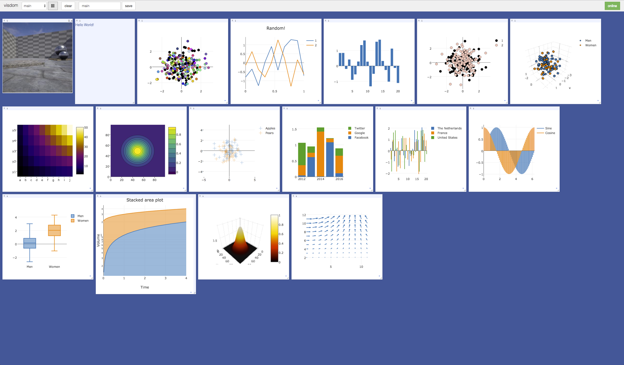
Windows

The UI begins as a blank slate â you can populate it with plots, images, and text. These appear in windows that you can drag, drop, resize, and destroy. The windows live in envs and the state of envs is stored across sessions. You can download the content of windows â including your plots in svg.

Tip: You can use the zoom of your browser to adjust the scale of the UI.

Callbacks

The python Visdom implementation supports callbacks on a window. The demo shows an example of this in the form of an editable text pad. The functionality of these callbacks allows the Visdom object to receive and react to events that happen in the frontend.

You can subscribe a window to events by adding a function to the event handlers dict for the window id you want to subscribe by calling viz.register_event_handler(handler, win_id) with your handler and the window id. Multiple handlers can be registered to the same window. You can remove all event handlers from a window using viz.clear_event_handlers(win_id). When an event occurs to that window, your callbacks will be called on a dict containing:

event_type: one of the below event types
pane_data: all of the stored contents for that window including layout and content.
eid: the current environment id
target: the window id the event is called on

Additional parameters are defined below.

Right now the following callback events are supported:

Close - Triggers when a window is closed. Returns a dict with only the aforementioned fields.
KeyPress - Triggers when a key is pressed. Contains additional parameters:
- key - A string representation of the key pressed (applying state modifiers such as SHIFT)
- key_code - The javascript event keycode for the pressed key (no modifiers)
PropertyUpdate - Triggers when a property is updated in Property pane
- propertyId - Position in properties list
- value - New property value
Click - Triggers when Image pane is clicked on, has a parameter:
- image_coord - dictionary with the fields x and y for the click coordinates in the coordinate frame of the possibly zoomed/panned image (not the enclosing pane).

Editable Plot Parameters

Use the top-right *edit*-Button to inspect all parameters used for plot in the respective window. The visdom client supports dynamic change of plot parameters as well. Just change one of the listed parameters, the plot will be altered on-the-fly. Click the button again to close the property list.

Environments

You can partition your visualization space with envs. By default, every user will have an env called main. New envs can be created in the UI or programmatically. The state of envs is chronically saved. Environments are able to keep entirely different pools of plots.

You can access a specific env via url: http://localhost.com:8097/env/main. If your server is hosted, you can share this url so others can see your visualizations too.

Environments are automatically hierarchically organized by the first _.

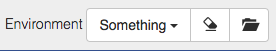
Selecting Environments

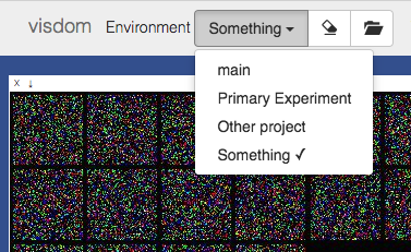
From the main page it is possible to toggle between different environments using the environment selector. Selecting a new environment will query the server for the plots that exist in that environment. The environment selector allows for searching and filtering for the new enironment.

Comparing Environments

From the main page it is possible to compare different environments using the environment selector. Selecting multiple environments in the check box will query the server for the plots with the same titles in all environments and plot them in a single plot. An additional compare legend pane is created with a number corresponding to each selected environment. Individual plots are updated with legends corresponding to "x_name" where x is a number corresponding with the compare legend pane and name is the original name in the legend.

Note: The compare envs view is not robust to high throughput data, as the server is responsible for generating the compared content. Do not compare an environment that is receiving a high quantity of updates on any plot, as every update will request regenerating the comparison. If you need to compare two plots that are receiving high quantities of data, have them share the same window on a singular env.

Clearing Environments

You can use the eraser button to remove all of the current contents of an environment. This closes the plot windows for that environment but keeps the empty environment for new plots.

Managing Environments

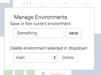
Pressing the folder icon opens a dialog that allows you to fork or force save the current environment, or delete any of your existing environments. Use of this feature is fully described in the State section.

Env Files: Your envs are loaded upon request by the user, by default from $HOME/.visdom/. Custom paths can be passed as a cmd-line argument. Envs are removed by using the delete button or by deleting the corresponding .json file from the env dir. In case you want the server to pre-load all files into cache, use the flag -eager_data_loading.

State

Once you've created a few visualizations, state is maintained. The server automatically caches your visualizations -- if you reload the page, your visualizations reappear.

Save: You can manually do so with the save button. This will serialize the env's state (to disk, in JSON), including window positions. You can save an env programmatically.
This is helpful for more sophisticated visualizations in which configuration is meaningful, e.g. a data-rich demo, a model training dashboard, or systematic experimentation. This also makes them easy to share and reuse.
Fork: If you enter a new env name, saving will create a new env -- effectively forking the previous env.

Tip: Fork an environment before you begin to make edits to ensure that your changes are saved seperately.

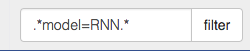
Filter

You can use the filter to dynamically sift through windows present in an env -- just provide a regular expression with which to match titles of window you want to show. This can be helpful in use cases involving an env with many windows e.g. when systematically checking experimental results.

Note: If you have saved your current view, the view will be restored after clearing the filter.

Views

It is possible to manage the views simply by dragging the tops of windows around, however additional features exist to keep views organized and save common views. View management can be useful for saving and switching between multiple common organizations of your windows.

Saving/Deleting Views

Using the folder icon, a dialog window opens where views can be forked in the same way that envs can be. Saving a view will retain the position and sizes of all of the windows in a given environment. Views are saved in $HOME/.visdom/view/layouts.json in the visdom filepath.

Note: Saved views are static, and editing a saved view copies that view over to the current view where editing can occur.

Re-Packing

Using the repack icon (9 boxes), visdom will attempt to pack your windows in a way that they best fit while retaining row/column ordering.

Note: Due to the reliance on row/column ordering and ReactGridLayout the final layout might be slightly different than what might be expected. We're working on improving that experience or providing alternatives that give more fine-tuned control.

Reloading Views

Using the view dropdown it is possible to select previously saved views, restoring the locations and sizes of all of the windows within the current environment to the places they were when that view was saved last.

Setup

Python and web clients come bundled with the python server.

Install from pip

> pip install visdom

Install from source

> pip install git+https://github.com/fossasia/visdom

Usage

Start the server (probably in a screen or tmux) from the command line:

> visdom

Visdom now can be accessed by going to http://localhost:8097 in your browser, or your own host address if specified.

The visdom command is equivalent to running python -m visdom.server.

If the above does not work, try using an SSH tunnel to your server by adding the following line to your local ~/.ssh/config: LocalForward 127.0.0.1:8097 127.0.0.1:8097.

Command Line Options

The following options can be provided to the server:

-port : The port to run the server on.
-hostname : The hostname to run the server on.
-base_url : The base server url (default = /).
-env_path : The path to the serialized session to reload.
-logging_level : Logging level (default = INFO). Accepts both standard text and numeric logging values.
-readonly : Flag to start server in readonly mode.
-enable_login : Flag to setup authentication for the sever, requiring a username and password to login.
-force_new_cookie : Flag to reset the secure cookie used by the server, invalidating current login cookies. Requires -enable_login.
-bind_local : Flag to make the server accessible only from localhost.
-eager_data_loading : By default visdom loads environments lazily upon user request. Setting this flag lets visdom pre-fetch all environments upon startup.

When -enable_login flag is provided, the server asks user to input credentials using terminal prompt. Alternatively, you can setup VISDOM_USE_ENV_CREDENTIALS env variable, and then provide your username and password via VISDOM_USERNAME and VISDOM_PASSWORD env variables without manually interacting with the terminal. This setup is useful in case if you would like to launch visdom server from bash script, or from Jupyter notebook.

VISDOM_USERNAME=username
VISDOM_PASSWORD=password
VISDOM_USE_ENV_CREDENTIALS=1 visdom -enable_login

You can also use VISDOM_COOKIE variable to provide cookies value if the cookie file wasn't generated, or the flag -force_new_cookie was set.

Python example

import visdom
import numpy as np
vis = visdom.Visdom()
vis.text('Hello, world!')
vis.image(np.ones((3, 10, 10)))

Demos

If you have cloned this repository, you can run our demo showcase.

python example/demo.py

API

For a quick introduction into the capabilities of visdom, have a look at the example directory, or read the details below.

Visdom Arguments (Python only)

The python visdom client takes a few options:

server: the hostname of your visdom server (default: 'http://localhost')
port: the port for your visdom server (default: 8097)
base_url: the base visdom server url (default: /)
env: Default environment to plot to when no env is provided (default: main)
raise_exceptions: Raise exceptions upon failure rather than printing them (default: True (soon))
log_to_filename: If not none, log all plotting and updating events to the given file (append mode) so that they can be replayed later using replay_log (default: None)
use_incoming_socket: enable use of the socket for receiving events from the web client, allowing user to register callbacks (default: True)
http_proxy_host: Deprecated. Use Proxies argument for complete proxy support.
http_proxy_port: Deprecated. Use Proxies argument for complete proxy support.
username: username to use for authentication, if server started with -enable_login (default: None)
password: password to use for authentication, if server started with -enable_login (default: None)
proxies: Dictionary mapping protocol to the URL of the proxy (e.g. {http: foo.bar:3128}) to be used on each Request. (default: None)
offline: Flag to run visdom in offline mode, where all requests are logged to file rather than to the server. Requires log_to_filename is set. In offline mode, all visdom commands that don't create or update plots will simply return True. (default: False)

Other options are either currently unused (endpoint, ipv6) or used for internal functionality.

Basics

Visdom offers the following basic visualization functions:

vis.image : image
vis.images : list of images
vis.text : arbitrary HTML
vis.properties : properties grid
vis.audio : audio
vis.video : videos
vis.svg : SVG object
vis.matplot : matplotlib plot
vis.save : serialize state server-side

Plotting

We have wrapped several common plot types to make creating basic visualizations easily. These visualizations are powered by Plotly.

The following API is currently supported:

vis.scatter : 2D or 3D scatter plots
vis.line : line plots
vis.stem : stem plots
vis.heatmap : heatmap plots
vis.bar : bar graphs
vis.histogram : histograms
vis.boxplot : boxplots
vis.surf : surface plots
vis.contour : contour plots
vis.quiver : quiver plots
vis.mesh : mesh plots
vis.dual_axis_lines : double y axis line plots

Generic Plots

Note that the server API adheres to the Plotly convention of data and layout objects, such that you can produce your own arbitrary Plotly visualizations:

import visdom
vis = visdom.Visdom()

trace = dict(x=[1, 2, 3], y=[4, 5, 6], mode="markers+lines", type='custom',
             marker={'color': 'red', 'symbol': 104, 'size': "10"},
             text=["one", "two", "three"], name='1st Trace')
layout = dict(title="First Plot", xaxis={'title': 'x1'}, yaxis={'title': 'x2'})

vis._send({'data': [trace], 'layout': layout, 'win': 'mywin'})

Others

vis.close : close a window by id
vis.delete_env : delete an environment by env_id
vis.win_exists : check if a window already exists by id
vis.get_env_list : get a list of all of the environments on your server
vis.get_window_data: get current data for a window
vis.check_connection: check if the server is connected
vis.replay_log: replay the actions from the provided log file

Details

Basics

vis.image

This function draws an img. It takes as input an CxHxW tensor img that contains the image.

The following opts are supported:

jpgquality: JPG quality (number 0-100). If defined image will be saved as JPG to reduce file size. If not defined image will be saved as PNG.
caption: Caption for the image
store_history: Keep all images stored to the same window and attach a slider to the bottom that will let you select the image to view. You must always provide this opt when sending new images to an image with history.

Note You can use alt on an image pane to view the x/y coordinates of the cursor. You can also ctrl-scroll to zoom, alt scroll to pan vertically, and alt-shift scroll to pan horizontally. Double click inside the pane to restore the image to default.

vis.images

This function draws a list of images. It takes an input B x C x H x W tensor or a list of images all of the same size. It makes a grid of images of size (B / nrow, nrow).

The following arguments and opts are supported:

nrow: Number of images in a row
padding: Padding around the image, equal padding around all 4 sides
opts.jpgquality: JPG quality (number 0-100). If defined image will be saved as JPG to reduce file size. If not defined image will be saved as PNG.
opts.caption: Caption for the image

vis.text

This function prints text in a box. You can use this to embed arbitrary HTML. It takes as input a text string. No specific opts are currently supported.

vis.properties

This function shows editable properties in a pane. Properties are expected to be a List of Dicts e.g.:

    properties = [
        {'type': 'text', 'name': 'Text input', 'value': 'initial'},
        {'type': 'number', 'name': 'Number input', 'value': '12'},
        {'type': 'button', 'name': 'Button', 'value': 'Start'},
        {'type': 'checkbox', 'name': 'Checkbox', 'value': True},
        {'type': 'select', 'name': 'Select', 'value': 1, 'values': ['Red', 'Green', 'Blue']},
    ]

Supported types:

text: string
number: decimal number
button: button labeled with "value"
checkbox: boolean value rendered as a checkbox
select: multiple values select box
- value: id of selected value (zero based)
- values: list of possible values

Callback are called on property value update:

event_type: "PropertyUpdate"
propertyId: position in the properties list
value: new value

No specific opts are currently supported.

vis.audio

This function plays audio. It takes as input the filename of the audio file or an N tensor containing the waveform (use an Nx2 matrix for stereo audio). The function does not support any plot-specific opts.

The following opts are supported:

opts.sample_frequency: sample frequency (integer > 0; default = 44100)

Known issue: Visdom uses scipy to convert tensor inputs to wave files. Some versions of Chrome are known not to play these wave files (Firefox and Safari work fine).

vis.video

This function plays a video. It takes as input the filename of the video videofile or a LxHxWxC-sized tensor containing all the frames of the video as input. The function does not support any plot-specific opts.

The following opts are supported:

opts.fps: FPS for the video (integer > 0; default = 25)

Note: Using tensor input requires that ffmpeg is installed and working. Your ability to play video may depend on the browser you use: your browser has to support the Theano codec in an OGG container (Chrome supports this).

vis.svg

This function draws an SVG object. It takes as input a SVG string svgstr or the name of an SVG file svgfile. The function does not support any specific opts.

vis.matplot

This function draws a Matplotlib plot. The function supports one plot-specific option: resizable.

Note When set to True the plot is resized with the pane. You need beautifulsoup4 and lxml packages installed to use this option.

Note: matplot is not rendered using the same backend as plotly plots, and is somewhat less efficient. Using too many matplot windows may degrade visdom performance.

vis.plotlyplot

This function draws a Plotly Figure object. It does not explicitly take options as it assumes you have already explicitly configured the figure's layout.

Note You must have the plotly Python package installed to use this function. It can typically be installed by running pip install plotly.

vis.embeddings

This function visualizes a collection of features using the Barnes-Hut t-SNE algorithm.

The function accepts the following arguments:

features: a list of tensors
labels: a list of corresponding labels for the tensors provided for features
data_getter=fn: (optional) a function that takes as a parameter an index into the features array and returns a summary representation of the tensor. If this is set, data_type must also be set.
data_type=str: (optional) currently the only acceptable value here is "html"

We currently assume that there are no more than 10 unique labels, in the future we hope to provide a colormap in opts for other cases.

From the UI you can also draw a lasso around a subset of features. This will rerun the t-SNE visualization on the selected subset.

vis.save

This function saves the envs that are alive on the visdom server. It takes input a list of env ids to be saved.

Plotting

Further details on the wrapped plotting functions are given below.

The exact inputs into the plotting functions vary, although most of them take as input a tensor X than contains the data and an (optional) tensor Y that contains optional data variables (such as labels or timestamps). All plotting functions take as input an optional win that can be used to plot into a specific window; each plotting function also returns the win of the window it plotted in. One can also specify the env to which the visualization should be added.

vis.scatter

This function draws a 2D or 3D scatter plot. It takes as input an Nx2 or Nx3 tensor X that specifies the locations of the N points in the scatter plot. An optional N tensor Y containing discrete labels that range between 1 and K can be specified as well -- the labels will be reflected in the colors of the markers.

update can be used to efficiently update the data of an existing plot. Use 'append' to append data, 'replace' to use new data, or 'remove' to remove the trace specified by name. Using update='append' will create a plot if it doesn't exist and append to the existing plot otherwise. If updating a single trace, use name to specify the name of the trace to be updated. Update data that is all NaN is ignored (can be used for masking update).

The following opts are supported:

opts.markersymbol : marker symbol (string; default = 'dot')
opts.markersize : marker size (number; default = '10')
opts.markercolor : color per marker. (torch.*Tensor; default = nil)
opts.markerborderwidth: marker border line width (float; default = 0.5)
opts.legend : table containing legend names
opts.textlabels : text label for each point (list: default = None)
opts.layoutopts : dict of any additional options that the graph backend accepts for a layout. For example layoutopts = {'plotly': {'legend': {'x':0, 'y':0}}}.
opts.traceopts : dict mapping trace names or indices to dicts of additional options that the graph backend accepts. For example traceopts = {'plotly': {'myTrace': {'mode': 'markers'}}}.
opts.webgl : use WebGL for plotting (boolean; default = false). It is faster if a plot contains too many points. Use sparingly as browsers won't allow more than a couple of WebGL contexts on a single page.

opts.markercolor is a Tensor with Integer values. The tensor can be of size N or N x 3 or K or K x 3.

Tensor of size N: Single intensity value per data point. 0 = black, 255 = red
Tensor of size N x 3: Red, Green and Blue intensities per data point. 0,0,0 = black, 255,255,255 = white
Tensor of size K and K x 3: Instead of having a unique color per data point, the same color is shared for all points of a particular label.

vis.sunburst

This function draws a sunburst chart. It takes two inputs: parents and labels array. values from parents array is used as parents object, like it define above which sector should the this sector shown. values from labels array is used to define sector's label or you can say name. keep in mind that lenght of array parents and labels should be equal. There is a third array that you can pass to which is value, it is use to show a value on hovering over a sector, it is optional argument, but if you are passing it then keep in mind lenght of values should be equal to parents or labels.

Following opts are currently supported:

opts.font_size : define font size of label (int)
opts.font_color : define font color of label (string)
opts.opacity : define opacity of chart (float)
opts.line_width : define distance between two sectors and sector to its parents (int)

vis.line

This function draws a line plot. It takes as input an N or NxM tensor Y that specifies the values of the M lines (that connect N points) to plot. It also takes an optional X tensor that specifies the corresponding x-axis values; X can be an N tensor (in which case all lines will share the same x-axis values) or have the same size as Y.

update can be used to efficiently update the data of an existing plot. Use 'append' to append data, 'replace' to use new data, or 'remove' to remove the trace specified by name. If updating a single trace, use name to specify the name of the trace to be updated. Update data that is all NaN is ignored (can be used for masking update).

Smoothing: Line plots can be smoothened using Savitzky-Golay filtering. This feature can be enabled by clicking the ~-symbol in the top right corner of a window that contains a line plot.

Demo of interactive smoothing.

The following opts are supported:

opts.fillarea : fill area below line (boolean)
opts.markers : show markers (boolean; default = false)
opts.markersymbol: marker symbol (string; default = 'dot')
opts.markersize : marker size (number; default = '10')
opts.linecolor : line colors (np.array; default = None)
opts.dash : line dash type for each line (np.array; default = 'solid'), one of solid, dash, dashdot or dash, size should match number of lines being drawn
opts.legend : table containing legend names
opts.layoutopts : dict of any additional options that the graph backend accepts for a layout. For example layoutopts = {'plotly': {'legend': {'x':0, 'y':0}}}.
opts.traceopts : dict mapping trace names or indices to dicts of additional options that plot.ly accepts for a trace.
opts.webgl : use WebGL for plotting (boolean; default = false). It is faster if a plot contains too many points. Use sparingly as browsers won't allow more than a couple of WebGL contexts on a single page.

vis.stem

This function draws a stem plot. It takes as input an N or NxM tensor X that specifies the values of the N points in the M time series. An optional N or NxM tensor Y containing timestamps can be specified as well; if Y is an N tensor then all M time series are assumed to have the same timestamps.

The following opts are supported:

opts.colormap: colormap (string; default = 'Viridis')
opts.legend : table containing legend names
opts.layoutopts : dict of any additional options that the graph backend accepts for a layout. For example layoutopts = {'plotly': {'legend': {'x':0, 'y':0}}}.

vis.heatmap

This function draws a heatmap. It takes as input an NxM tensor X that specifies the value at each location in the heatmap.

update can be used to efficiently update the data of an existing plot. Use 'appendRow' to append data row-wise, 'appendColumn' to append data column-wise, 'prependRow' to prepend data row-wise, 'prependColumn' to prepend data column-wise, 'replace' to use new data, or 'remove' to remove the plot specified by win.

The following opts are supported:

opts.colormap : colormap (string; default = 'Viridis')
opts.xmin : clip minimum value (number; default = X:min())
opts.xmax : clip maximum value (number; default = X:max())
opts.columnnames: table containing x-axis labels
opts.rownames : table containing y-axis labels
opts.layoutopts : dict of any additional options that the graph backend accepts for a layout. For example layoutopts = {'plotly': {'legend': {'x':0, 'y':0}}}.
opts.nancolor : color for plotting NaNs. If this is None, NaNs will be plotted as transparent. (string; default = None)

vis.bar

This function draws a regular, stacked, or grouped bar plot. It takes as input an N or NxM tensor X that specifies the height of each of the bars. If X contains M columns, the values corresponding to each row are either stacked or grouped (depending on how opts.stacked is set). In addition to X, an (optional) N tensor Y can be specified that contains the corresponding x-axis values.

The following plot-specific opts are currently supported:

opts.rownames: table containing x-axis labels
opts.stacked : stack multiple columns in X
opts.legend : table containing legend labels
opts.layoutopts : dict of any additional options that the graph backend accepts for a layout. For example layoutopts = {'plotly': {'legend': {'x':0, 'y':0}}}.

vis.histogram

This function draws a histogram of the specified data. It takes as input an N tensor X that specifies the data of which to construct the histogram.

The following plot-specific opts are currently supported:

opts.numbins: number of bins (number; default = 30)
opts.layoutopts : dict of any additional options that the graph backend accepts for a layout. For example layoutopts = {'plotly': {'legend': {'x':0, 'y':0}}}.

vis.boxplot

This function draws boxplots of the specified data. It takes as input an N or an NxM tensor X that specifies the N data values of which to construct the M boxplots.

The following plot-specific opts are currently supported:

opts.legend: labels for each of the columns in X
opts.layoutopts : dict of any additional options that the graph backend accepts for a layout. For example layoutopts = {'plotly': {'legend': {'x':0, 'y':0}}}.

vis.surf

This function draws a surface plot. It takes as input an NxM tensor X that specifies the value at each location in the surface plot.

The following opts are supported:

opts.colormap: colormap (string; default = 'Viridis')
opts.xmin : clip minimum value (number; default = X:min())
opts.xmax : clip maximum value (number; default = X:max())
opts.layoutopts : dict of any additional options that the graph backend accepts for a layout. For example layoutopts = {'plotly': {'legend': {'x':0, 'y':0}}}.

vis.contour

This function draws a contour plot. It takes as input an NxM tensor X that specifies the value at each location in the contour plot.

The following opts are supported:

opts.colormap: colormap (string; default = 'Viridis')
opts.xmin : clip minimum value (number; default = X:min())
opts.xmax : clip maximum value (number; default = X:max())
opts.layoutopts : dict of any additional options that the graph backend accepts for a layout. For example layoutopts = {'plotly': {'legend': {'x':0, 'y':0}}}.

vis.quiver

This function draws a quiver plot in which the direction and length of the arrows is determined by the NxM tensors X and Y. Two optional NxM tensors gridX and gridY can be provided that specify the offsets of the arrows; by default, the arrows will be done on a regular grid.

The following opts are supported:

opts.normalize: length of longest arrows (number)
opts.arrowheads: show arrow heads (boolean; default = true)
opts.layoutopts : dict of any additional options that the graph backend accepts for a layout. For example layoutopts = {'plotly': {'legend': {'x':0, 'y':0}}}.

vis.mesh

This function draws a mesh plot from a set of vertices defined in an Nx2 or Nx3 matrix X, and polygons defined in an optional Mx2 or Mx3 matrix Y.

The following opts are supported:

opts.color: color (string)
opts.opacity: opacity of polygons (number between 0 and 1)
opts.layoutopts : dict of any additional options that the graph backend accepts for a layout. For example layoutopts = {'plotly': {'legend': {'x':0, 'y':0}}}.

vis.dual_axis_lines

This function will create a line plot using plotly with different Y-Axis.

X = A numpy array of the range.

Y1 = A numpy array of the same count as X.

Y2 = A numpy array of the same count as X.

The following opts are supported:

opts.height : Height of the plot
opts.width : Width of the plot
opts.name_y1 : Axis name for Y1 plot
opts.name_y2 : Axis name for Y2 plot
opts.title : Title of the plot
opts.color_title_y1 : Color of the Y1 axis Title
opts.color_tick_y1 : Color of the Y1 axis Ticks
opts.color_title_y2 : Color of the Y2 axis Title
opts.color_tick_y2 : Color of the Y2 axis Ticks
opts.side : side on which the Y2 tick has to be placed. Has values 'right' or left.
opts.showlegend : Display legends (boolean values)
opts.top : Set the top margin of the plot
opts.bottom : Set the bottom margin of the plot
opts.right : Set the right margin of the plot
opts.left : Set the left margin of the plot

This is the image of the output:

Network Graph

This function draws a graph, in which the nodes and edges are taken from a 2-D matrix of size [,2] where each row contains a source and destination node value. The numeric value used to define nodes should be strictly between (0 to n-1), where n is the number of nodes.

There are two optional arguments :

edgeLabels : list of custom edge labels. If not provided each edge gets a label, "source-destination", eg "1-2", size should be equal to size of input "edges". Optional.
nodeLabels : list of custom node labels. If not provided each node gets a label same as the numeric value defined in the "edges". size should be equal to number of nodes present. Optional.

The following opts are supported:

opts.height : Height of the plot. Default : 500
opts.width : Width of the plot. Default : 500
opts.directed : whether the plot should have a arrow or not. Default : false
opts.showVertexLabels : Whether to show vertex labels. Default : true
opts.showEdgeLabels : Whether to show edge labels. Default : false
opts.scheme : Whether all nodes shoud have "same" color or "different". Default : "same"

Customizing plots

The plotting functions take an optional opts table as input that can be used to change (generic or plot-specific) properties of the plots.

All input arguments are specified in a single table; the input arguments are matches based on the keys they have in the input table.

The following opts are generic in the sense that they are the same for all visualizations (except plot.image, plot.text, plot.video, and plot.audio):

opts.title : figure title
opts.width : figure width
opts.height : figure height
opts.showlegend : show legend (true or false)
opts.xtype : type of x-axis ('linear' or 'log')
opts.xlabel : label of x-axis
opts.xtick : show ticks on x-axis (boolean)
opts.xtickmin : first tick on x-axis (number)
opts.xtickmax : last tick on x-axis (number)
opts.xtickvals : locations of ticks on x-axis (table of numbers)
opts.xticklabels : ticks labels on x-axis (table of strings)
opts.xtickstep : distances between ticks on x-axis (number)
opts.xtickfont : font for x-axis labels (dict of font information)
opts.ytype : type of y-axis ('linear' or 'log')
opts.ylabel : label of y-axis
opts.ytick : show ticks on y-axis (boolean)
opts.ytickmin : first tick on y-axis (number)
opts.ytickmax : last tick on y-axis (number)
opts.ytickvals : locations of ticks on y-axis (table of numbers)
opts.yticklabels : ticks labels on y-axis (table of strings)
opts.ytickstep : distances between ticks on y-axis (number)
opts.ytickfont : font for y-axis labels (dict of font information)
opts.marginleft : left margin (in pixels)
opts.marginright : right margin (in pixels)
opts.margintop : top margin (in pixels)
opts.marginbottom: bottom margin (in pixels)

opts are passed as dictionary in python scripts.You can pass opts like:

opts=dict(title="my title", xlabel="x axis",ylabel="y axis")

opts={"title":"my title", "xlabel":"x axis","ylabel":"y axis"}

The other options are visualization-specific, and are described in the documentation of the functions.

Others

vis.close

This function closes a specific window. It takes input window id win and environment id eid. Use win as None to close all windows in an environment.

vis.delete_env

This function deletes a specified env entirely. It takes env id eid as input.

Note: delete_env is deletes all data for an environment and is IRREVERSIBLE. Do not use unless you absolutely want to remove an environment.

vis.fork_env

This function forks an environment, similiar to the UI feature.

Arguments:

prev_eid: Environment ID that we want to fork.
eid: New Environment ID that will be created with the fork.

Note: fork_env an exception will occur if an env that doesn't exist is forked.

vis.win_exists

This function returns a bool indicating whether or not a window win exists on the server already. Returns None if something went wrong.

Optional arguments:

env: Environment to search for the window in. Default is None.

vis.get_env_list

This function returns a list of all of the environments on the server at the time of calling. It takes no arguments.

vis.get_window_data

This function returns the window data for the given window. Returns data for all windows in an env if win is None.

Arguments:

env: Environment to search for the window in.
win: Window to return data for. Set to None to retrieve all the windows in an environment.

vis.check_connection

This function returns a bool indicating whether or not the server is connected. It accepts an optional argument timeout_seconds for a number of seconds to wait for the server to come up.

vis.replay_log

This function takes the contents of a visdom log and replays them to the current server to restore a state or handle any missing entries.

Arguments:

log_filename: log file to replay the contents of.

Customizing Visdom

The user config directory for visdom is

~/.config/visdom for Linux
~/Library/Preferences/visdom for OSX
%APPDATA%/visdom for Windows

By placing a style.css in you user config directory, visdom will serve the customized css file along with the default style-file. In addition, it is also possible to create a project-specific file; just place the file style.css in your env_path.

License

visdom is Apache 2.0 licensed, as found in the LICENSE file.

Note on Lua Torch Support

Support for Lua Torch was deprecated following v0.1.8.4. If you'd like to use torch support, you'll need to download that release. You can follow the usage instructions there, but it is no longer officially supported.

Contributing

See guidelines for contributing here.

Acknowledgments

Visdom was inspired by tools like display and relies on Plotly as a plotting front-end.

Top Related Projects

Convert designs to code with AI

Introducing Visual Copilot: A new AI model to turn Figma designs to high quality code using your components.

Try Visual Copilot