Top Related Projects
A general-purpose tool for dynamic report generation in R
Jupyter metapackage for installation, docs and chat
Jupyter Notebooks as Markdown Documents, Julia, Python or R scripts
Create beautiful, publication-quality books and documents from computational content.
Static site generator that supports Markdown and reST syntax. Powered by Python.
Quick Overview
RStudio's rmarkdown is a powerful R package that enables dynamic report generation, combining R code, its output, and narrative text. It allows users to create reproducible documents in various formats, including HTML, PDF, and Word, using a simple markdown syntax enhanced with R code chunks.
Pros
- Seamless integration of code, output, and narrative text
- Supports multiple output formats (HTML, PDF, Word, etc.)
- Highly customizable with various options and themes
- Excellent for reproducible research and data analysis reports
Cons
- Learning curve for users new to R or markdown
- Rendering can be slow for large documents or complex analyses
- Some advanced features require additional LaTeX knowledge for PDF output
- Occasional compatibility issues with certain R packages or system configurations
Code Examples
- Basic R Markdown code chunk:
```{r}
# Create a simple plot
plot(mtcars$mpg, mtcars$hp,
     xlab = "Miles per Gallon",
     ylab = "Horsepower",
     main = "MPG vs Horsepower")
2. Customizing chunk options:

```r
```{r, echo=FALSE, fig.width=8, fig.height=6}
library(ggplot2)
ggplot(mtcars, aes(x = mpg, y = hp)) +
  geom_point() +
  geom_smooth(method = "lm") +
  labs(title = "MPG vs Horsepower",
       x = "Miles per Gallon",
       y = "Horsepower")
3. Including inline R code:

```markdown
The average miles per gallon in the mtcars dataset is `r round(mean(mtcars$mpg), 2)`.
Getting Started
- Install the rmarkdown package:
install.packages("rmarkdown")
-
Create a new R Markdown file in RStudio:
- File > New File > R Markdown
- Choose a document type (e.g., HTML, PDF, Word)
-
Write your content using markdown syntax and R code chunks
-
Click the "Knit" button in RStudio to render the document
For more advanced usage, refer to the R Markdown documentation.
Competitor Comparisons
A general-purpose tool for dynamic report generation in R
Pros of knitr
- More flexible and customizable for advanced users
- Supports a wider range of programming languages
- Offers finer control over code chunk options and output
Cons of knitr
- Steeper learning curve for beginners
- Less integrated with RStudio IDE features
- Requires more manual configuration for complex documents
Code Comparison
knitr:
<<chunk-name, echo=FALSE, results='asis'>>=
cat("This is a knitr code chunk")
@
rmarkdown:
```{r chunk-name, echo=FALSE, results='asis'}
cat("This is an R Markdown code chunk")
Summary
knitr is a powerful and flexible engine for dynamic report generation, offering more advanced features and language support. However, it may be more challenging for beginners and requires more manual setup. rmarkdown, built on top of knitr, provides a more user-friendly interface and better integration with RStudio, making it easier for newcomers to create dynamic documents. The choice between the two depends on the user's needs, experience level, and desired level of control over the document generation process.
Jupyter metapackage for installation, docs and chat
Pros of Jupyter
- Supports multiple programming languages (Python, R, Julia, etc.)
- Interactive, cell-based execution model
- Rich media output (plots, images, videos) inline
Cons of Jupyter
- Less integrated with version control systems
- Can be challenging to reproduce entire workflows
- Limited built-in options for creating polished reports
Code Comparison
Jupyter notebook cell:
import matplotlib.pyplot as plt
plt.plot([1, 2, 3, 4])
plt.ylabel('some numbers')
plt.show()
RMarkdown chunk:
library(ggplot2)
ggplot(data.frame(x=1:4, y=1:4), aes(x, y)) +
  geom_line() +
  ylab('some numbers')
Both Jupyter and RMarkdown offer powerful tools for data analysis and reporting. Jupyter excels in interactive exploration and supports multiple languages, making it versatile for various data science tasks. RMarkdown, while primarily focused on R, provides a more streamlined experience for creating reproducible reports and integrates well with version control systems. The choice between the two often depends on the specific needs of the project and the preferred programming language.
Jupyter Notebooks as Markdown Documents, Julia, Python or R scripts
Pros of Jupytext
- Language-agnostic, supporting multiple programming languages beyond R
- Allows version control of notebooks in plain text formats (e.g., Markdown, R Markdown)
- Seamless integration with Jupyter environments
Cons of Jupytext
- Less integrated with RStudio IDE compared to R Markdown
- May require additional setup and configuration for optimal use
- Limited built-in rendering options compared to R Markdown's extensive output formats
Code Comparison
R Markdown:
---
title: "My Document"
output: html_document
---

```{r}
print("Hello, R Markdown!")
Jupytext:

```python
# ---
# title: My Document
# ---

# %%
print("Hello, Jupytext!")
Key Differences
- R Markdown uses YAML headers for metadata, while Jupytext uses commented YAML
- R Markdown has specific code chunk syntax, Jupytext uses cell markers (e.g.,
# %%) - R Markdown is primarily designed for R, while Jupytext supports multiple languages
- Jupytext focuses on version control and interoperability, R Markdown on document generation
Create beautiful, publication-quality books and documents from computational content.
Pros of Jupyter Book
- Supports multiple programming languages, not limited to R
- Designed for creating entire books and websites, with built-in navigation and structure
- Integrates well with Jupyter notebooks and the broader Jupyter ecosystem
Cons of Jupyter Book
- Steeper learning curve, especially for users not familiar with Jupyter
- Less seamless integration with RStudio IDE
- May require more setup and configuration for complex projects
Code Comparison
Jupyter Book:
# _toc.yml
format: jb-book
root: intro
chapters:
  - file: chapter1
  - file: chapter2
RMarkdown:
# _bookdown.yml
book_filename: "my_book"
language:
  ui:
    chapter_name: "Chapter "
output_dir: "docs"
Both systems use YAML configuration files, but Jupyter Book's structure is more focused on defining the book's table of contents, while RMarkdown's configuration is more about output settings and general book properties.
Static site generator that supports Markdown and reST syntax. Powered by Python.
Pros of Pelican
- Written in Python, making it more accessible for Python developers
- Supports multiple content formats including reStructuredText and HTML
- Highly extensible with a rich plugin ecosystem
Cons of Pelican
- Lacks built-in support for interactive elements and data analysis
- Steeper learning curve for non-Python users
- Limited real-time preview capabilities compared to RMarkdown
Code Comparison
Pelican (Python):
from pelican import Pelican
from pelican.settings import read_settings

settings = read_settings('pelicanconf.py')
pelican = Pelican(settings)
pelican.run()
RMarkdown (R):
library(rmarkdown)
render("input.Rmd", output_format = "html_document")
Both Pelican and RMarkdown are powerful static site generators, but they cater to different audiences. Pelican is more suited for Python developers and offers flexibility in content formats, while RMarkdown excels in creating interactive, data-driven documents within the R ecosystem. The choice between them often depends on the user's programming background and specific project requirements.
Convert  designs to code with AI

Introducing Visual Copilot: A new AI model to turn Figma designs to high quality code using your components.
Try Visual CopilotREADME
rmarkdown 
The rmarkdown package helps you create dynamic analysis documents that combine code, rendered output (such as figures), and prose. You bring your data, code, and ideas, and R Markdown renders your content into a polished document that can be used to:
-
Do data science interactively within the RStudio IDE,
-
Reproduce your analyses,
-
Collaborate and share code with others, and
-
Communicate your results with others.
R Markdown documents can be rendered to many output formats including HTML documents, PDFs, Word files, slideshows, and more, allowing you to focus on the content while R Markdown takes care of your presentation.
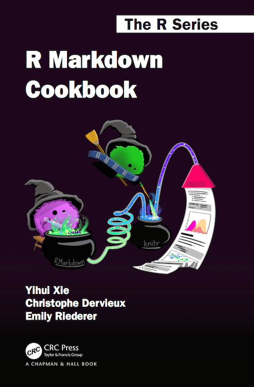
Books
See more about them in Get Started.
Installation
The easiest way to install the rmarkdown package is from within the RStudio IDE, but you don't need to explicitly install it or load it, as RStudio automatically does both when needed. A recent version of Pandoc (>= 1.12.3) is also required; RStudio also automatically includes this too so you do not need to download Pandoc if you plan to use rmarkdown from the RStudio IDE.
If you want to use the rmarkdown package outside of RStudio, you can install the package from CRAN as follows:
install.packages("rmarkdown")
If you want to use the development version of the rmarkdown package (either with or without RStudio), you can install the package from GitHub via the pak package:
# install.packages("pak")
pak::pak('rstudio/rmarkdown')
If not using the RStudio IDE, you'll need to install a recent version of Pandoc (>= 1.12.3); see the Pandoc installation instructions for help.
Usage
The easiest way to make a new R Markdown document is from within RStudio. Go to File > New File > R Markdown. From the new file wizard, you may:
- Provide a document title (optional but recommended),
- Provide an author name (optional but recommended),
- Select a default output format- HTML is the recommended format for authoring, and you can switch the output format anytime (required),
- Click OK (required).
Once inside your new .Rmd file, you should see some boilerplate text that includes code chunks. Use the "Knit" button in the RStudio IDE to render the file and preview the output with a single click or use the keyboard shortcut Cmd/Ctrl + Shift + K.
You can also delete all the text below the YAML frontmatter and fill in your own .Rmd by:
- Adding code chunks (keyboard shortcut:
Ctrl + Alt + I; OS X:Cmd + Option + I), - Writing prose with Markdown formatting, and
- Running each code chunk interactively by clicking the
 icon within RStudio.
You can also click "Knit to HTML" again to render the full document with all code chunks. For more help getting started in R Markdown, please see the R Markdown website or use the "Get Started" links at the top of this page.
Getting help
There are two main places to get help:
-
The Posit community is a friendly place to ask any questions about rmarkdown and the R Markdown family of packages.
-
Stack Overflow is a great source of answers to common rmarkdown questions. It is also a great place to get help, once you have created a reproducible example that illustrates your problem.
Code of Conduct
Please note that the rmarkdown project is released with a Contributor Code of Conduct. By contributing to this project, you agree to abide by its terms.
Top Related Projects
A general-purpose tool for dynamic report generation in R
Jupyter metapackage for installation, docs and chat
Jupyter Notebooks as Markdown Documents, Julia, Python or R scripts
Create beautiful, publication-quality books and documents from computational content.
Static site generator that supports Markdown and reST syntax. Powered by Python.
Convert  designs to code with AI

Introducing Visual Copilot: A new AI model to turn Figma designs to high quality code using your components.
Try Visual Copilot
