Top Related Projects
Flexible and powerful data analysis / manipulation library for Python, providing labeled data structures similar to R data.frame objects, statistical functions, and much more
Apache Spark - A unified analytics engine for large-scale data processing
R's data.table package extends data.frame:
The interactive graphing library for Python :sparkles:
Apache Arrow is the universal columnar format and multi-language toolbox for fast data interchange and in-memory analytics
Quick Overview
dplyr is a powerful R package for data manipulation and transformation. It provides a set of intuitive and consistent functions that make working with data frames and tibbles more efficient and readable. dplyr is part of the tidyverse ecosystem, which is designed to make data science workflows in R more coherent and streamlined.
Pros
- Intuitive and consistent syntax for data manipulation tasks
- Efficient performance, especially for large datasets
- Seamless integration with other tidyverse packages
- Extensive documentation and community support
Cons
- Learning curve for users coming from base R or other data manipulation paradigms
- Some functions may have unexpected behavior with certain data types
- Occasional breaking changes between major versions
- Dependency on the tidyverse ecosystem, which may not be ideal for all projects
Code Examples
- Basic data manipulation:
library(dplyr)

# Filter rows and select columns
mtcars %>%
  filter(mpg > 20) %>%
  select(mpg, cyl, wt)
- Grouping and summarizing data:
library(dplyr)

# Group by cylinder and calculate mean mpg
mtcars %>%
  group_by(cyl) %>%
  summarize(mean_mpg = mean(mpg))
- Joining data frames:
library(dplyr)

# Create sample data frames
df1 <- tibble(id = 1:3, value = c("a", "b", "c"))
df2 <- tibble(id = 2:4, score = c(80, 90, 100))

# Perform a left join
left_join(df1, df2, by = "id")
Getting Started
To get started with dplyr, follow these steps:
- Install the package:
install.packages("dplyr")
- Load the library:
library(dplyr)
- Use dplyr functions with the pipe operator:
mtcars %>%
  filter(mpg > 20) %>%
  select(mpg, cyl, wt) %>%
  arrange(desc(mpg))
This example filters cars with mpg > 20, selects specific columns, and sorts by mpg in descending order. Explore more functions like mutate(), summarize(), and group_by() to unlock the full potential of dplyr for your data manipulation tasks.
Competitor Comparisons
Flexible and powerful data analysis / manipulation library for Python, providing labeled data structures similar to R data.frame objects, statistical functions, and much more
Pros of pandas
- More comprehensive data manipulation library with extensive functionality
- Better performance for large datasets due to optimized C extensions
- Wider adoption in the data science and machine learning communities
Cons of pandas
- Steeper learning curve due to more complex API
- Less consistent syntax across different operations
- Slower development cycle compared to dplyr
Code Comparison
pandas:
import pandas as pd

df = pd.read_csv('data.csv')
result = df[df['column'] > 5].groupby('category').agg({'value': 'mean'})
dplyr:
library(dplyr)

df <- read_csv('data.csv')
result <- df %>%
  filter(column > 5) %>%
  group_by(category) %>%
  summarize(mean_value = mean(value))
Both libraries offer powerful data manipulation capabilities, but dplyr focuses on a more intuitive and consistent syntax using the pipe operator, while pandas provides a broader range of functionality at the cost of a more complex API. The choice between them often depends on the user's programming language preference (R vs Python) and specific project requirements.
Apache Spark - A unified analytics engine for large-scale data processing
Pros of Spark
- Designed for big data processing and distributed computing
- Supports multiple programming languages (Scala, Java, Python, R)
- Offers in-memory processing for faster performance
Cons of Spark
- Steeper learning curve and more complex setup
- Higher resource requirements for small-scale data processing
- Less intuitive for simple data manipulation tasks
Code Comparison
dplyr:
library(dplyr)
data %>%
  filter(column1 > 10) %>%
  group_by(column2) %>%
  summarize(mean_value = mean(column3))
Spark:
from pyspark.sql import SparkSession
from pyspark.sql.functions import mean

spark = SparkSession.builder.appName("example").getOrCreate()
data = spark.read.csv("data.csv", header=True, inferSchema=True)
result = data.filter(data.column1 > 10) \
             .groupBy("column2") \
             .agg(mean("column3").alias("mean_value"))
Summary
dplyr is more user-friendly for small to medium-sized datasets and simple data manipulation tasks, while Spark excels in processing large-scale data and distributed computing environments. dplyr offers a more intuitive syntax for R users, whereas Spark provides flexibility across multiple programming languages and advanced big data processing capabilities.
R's data.table package extends data.frame:
Pros of data.table
- Faster performance, especially for large datasets
- More memory-efficient operations
- Concise syntax for complex data manipulations
Cons of data.table
- Steeper learning curve due to unique syntax
- Less intuitive for beginners compared to dplyr's verb-based approach
- Fewer built-in functions for common data analysis tasks
Code Comparison
dplyr:
library(dplyr)
result <- mtcars %>%
  group_by(cyl) %>%
  summarize(avg_mpg = mean(mpg))
data.table:
library(data.table)
dt <- as.data.table(mtcars)
result <- dt[, .(avg_mpg = mean(mpg)), by = cyl]
Both dplyr and data.table are powerful R packages for data manipulation. dplyr offers a more intuitive, verb-based syntax that's easier for beginners to grasp, while data.table provides superior performance for large datasets and more concise syntax for complex operations. The choice between them often depends on the specific needs of the project, dataset size, and the user's familiarity with each package's syntax.
The interactive graphing library for Python :sparkles:
Pros of plotly.py
- Interactive and dynamic visualizations
- Supports a wide range of chart types
- Can be used in web applications and Jupyter notebooks
Cons of plotly.py
- Steeper learning curve for beginners
- Slower performance for large datasets
- Less integrated with data manipulation tasks
Code Comparison
dplyr:
library(dplyr)
mtcars %>%
  group_by(cyl) %>%
  summarize(avg_mpg = mean(mpg))
plotly.py:
import plotly.express as px
import pandas as pd

df = pd.read_csv('mtcars.csv')
fig = px.scatter(df, x='mpg', y='wt', color='cyl')
fig.show()
Key Differences
- dplyr focuses on data manipulation, while plotly.py specializes in visualization
- dplyr is part of the tidyverse ecosystem, offering seamless integration with other R packages
- plotly.py provides interactive plots out-of-the-box, whereas dplyr requires additional libraries for visualization
Use Cases
- dplyr: Ideal for data cleaning, transformation, and analysis tasks
- plotly.py: Best suited for creating interactive and shareable visualizations, especially for web applications
Apache Arrow is the universal columnar format and multi-language toolbox for fast data interchange and in-memory analytics
Pros of Arrow
- Designed for efficient processing of large-scale data across multiple languages and platforms
- Supports in-memory and on-disk data processing with optimized performance
- Provides zero-copy reads and interprocess communication for faster data transfer
Cons of Arrow
- Steeper learning curve compared to dplyr's intuitive syntax
- Less extensive ecosystem of helper functions and extensions
- May be overkill for smaller datasets or simpler data manipulation tasks
Code Comparison
dplyr:
library(dplyr)
data %>%
  filter(column1 > 10) %>%
  group_by(column2) %>%
  summarize(mean_value = mean(column3))
Arrow:
library(arrow)
open_dataset("path/to/data") %>%
  filter(column1 > 10) %>%
  group_by(column2) %>%
  summarize(mean_value = mean(column3)) %>%
  collect()
The Arrow code is similar to dplyr but operates on larger datasets efficiently. The collect() function is used to materialize the results in memory.
Convert  designs to code with AI

Introducing Visual Copilot: A new AI model to turn Figma designs to high quality code using your components.
Try Visual CopilotREADME
dplyr 
Overview
dplyr is a grammar of data manipulation, providing a consistent set of verbs that help you solve the most common data manipulation challenges:
mutate()adds new variables that are functions of existing variablesselect()picks variables based on their names.filter()picks cases based on their values.summarise()reduces multiple values down to a single summary.arrange()changes the ordering of the rows.
These all combine naturally with group_by() which allows you to
perform any operation âby groupâ. You can learn more about them in
vignette("dplyr"). As well as these single-table verbs, dplyr also
provides a variety of two-table verbs, which you can learn about in
vignette("two-table").
If you are new to dplyr, the best place to start is the data transformation chapter in R for Data Science.
Backends
In addition to data frames/tibbles, dplyr makes working with other computational backends accessible and efficient. Below is a list of alternative backends:
-
arrow for larger-than-memory datasets, including on remote cloud storage like AWS S3, using the Apache Arrow C++ engine, Acero.
-
dtplyr for large, in-memory datasets. Translates your dplyr code to high performance data.table code.
-
dbplyr for data stored in a relational database. Translates your dplyr code to SQL.
-
duckplyr for using duckdb on large, in-memory datasets with zero extra copies. Translates your dplyr code to high performance duckdb queries with an automatic R fallback when translation isnât possible.
-
duckdb for large datasets that are still small enough to fit on your computer.
-
sparklyr for very large datasets stored in Apache Spark.
Installation
# The easiest way to get dplyr is to install the whole tidyverse:
install.packages("tidyverse")

# Alternatively, install just dplyr:
install.packages("dplyr")
Development version
To get a bug fix or to use a feature from the development version, you can install the development version of dplyr from GitHub.
# install.packages("pak")
pak::pak("tidyverse/dplyr")
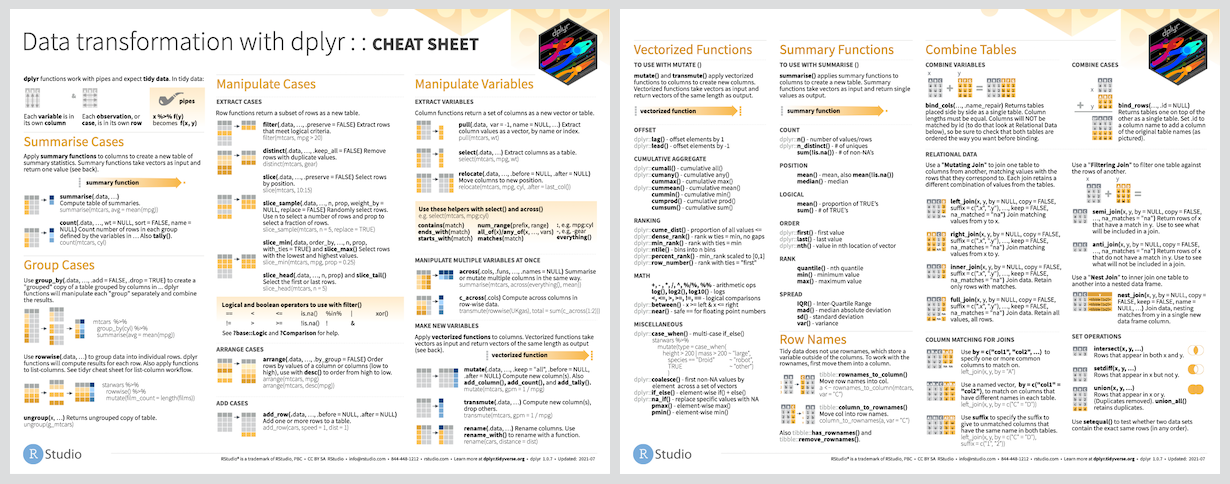
Cheat Sheet
Usage
library(dplyr)
starwars %>%
filter(species == "Droid")
#> # A tibble: 6 Ã 14
#> name height mass hair_color skin_color eye_color birth_year sex gender
#> <chr> <int> <dbl> <chr> <chr> <chr> <dbl> <chr> <chr>
#> 1 C-3PO 167 75 <NA> gold yellow 112 none masculiâ¦
#> 2 R2-D2 96 32 <NA> white, blue red 33 none masculiâ¦
#> 3 R5-D4 97 32 <NA> white, red red NA none masculiâ¦
#> 4 IG-88 200 140 none metal red 15 none masculiâ¦
#> 5 R4-P17 96 NA none silver, red red, blue NA none feminine
#> # â¹ 1 more row
#> # â¹ 5 more variables: homeworld <chr>, species <chr>, films <list>,
#> # vehicles <list>, starships <list>
starwars %>%
select(name, ends_with("color"))
#> # A tibble: 87 Ã 4
#> name hair_color skin_color eye_color
#> <chr> <chr> <chr> <chr>
#> 1 Luke Skywalker blond fair blue
#> 2 C-3PO <NA> gold yellow
#> 3 R2-D2 <NA> white, blue red
#> 4 Darth Vader none white yellow
#> 5 Leia Organa brown light brown
#> # â¹ 82 more rows
starwars %>%
mutate(name, bmi = mass / ((height / 100) ^ 2)) %>%
select(name:mass, bmi)
#> # A tibble: 87 Ã 4
#> name height mass bmi
#> <chr> <int> <dbl> <dbl>
#> 1 Luke Skywalker 172 77 26.0
#> 2 C-3PO 167 75 26.9
#> 3 R2-D2 96 32 34.7
#> 4 Darth Vader 202 136 33.3
#> 5 Leia Organa 150 49 21.8
#> # â¹ 82 more rows
starwars %>%
arrange(desc(mass))
#> # A tibble: 87 Ã 14
#> name height mass hair_color skin_color eye_color birth_year sex gender
#> <chr> <int> <dbl> <chr> <chr> <chr> <dbl> <chr> <chr>
#> 1 Jabba De⦠175 1358 <NA> green-tan⦠orange 600 herm⦠mascuâ¦
#> 2 Grievous 216 159 none brown, wh⦠green, y⦠NA male mascuâ¦
#> 3 IG-88 200 140 none metal red 15 none mascuâ¦
#> 4 Darth Va⦠202 136 none white yellow 41.9 male mascuâ¦
#> 5 Tarfful 234 136 brown brown blue NA male mascuâ¦
#> # â¹ 82 more rows
#> # â¹ 5 more variables: homeworld <chr>, species <chr>, films <list>,
#> # vehicles <list>, starships <list>
starwars %>%
group_by(species) %>%
summarise(
n = n(),
mass = mean(mass, na.rm = TRUE)
) %>%
filter(
n > 1,
mass > 50
)
#> # A tibble: 9 Ã 3
#> species n mass
#> <chr> <int> <dbl>
#> 1 Droid 6 69.8
#> 2 Gungan 3 74
#> 3 Human 35 81.3
#> 4 Kaminoan 2 88
#> 5 Mirialan 2 53.1
#> # â¹ 4 more rows
Getting help
If you encounter a clear bug, please file an issue with a minimal reproducible example on GitHub. For questions and other discussion, please use forum.posit.co.
Code of conduct
Please note that this project is released with a Contributor Code of Conduct. By participating in this project you agree to abide by its terms.
Top Related Projects
Flexible and powerful data analysis / manipulation library for Python, providing labeled data structures similar to R data.frame objects, statistical functions, and much more
Apache Spark - A unified analytics engine for large-scale data processing
R's data.table package extends data.frame:
The interactive graphing library for Python :sparkles:
Apache Arrow is the universal columnar format and multi-language toolbox for fast data interchange and in-memory analytics
Convert  designs to code with AI

Introducing Visual Copilot: A new AI model to turn Figma designs to high quality code using your components.
Try Visual Copilot