Top Related Projects
NeRF (Neural Radiance Fields) and NeRF in the Wild using pytorch-lightning
A PyTorch implementation of NeRF (Neural Radiance Fields) that reproduces the results.
Instant neural graphics primitives: lightning fast NeRF and more
PyTorch3D is FAIR's library of reusable components for deep learning with 3D data
Google Research
Plenoxels: Radiance Fields without Neural Networks
Quick Overview
bmild/nerf is a GitHub repository implementing Neural Radiance Fields (NeRF), a novel view synthesis technique. NeRF represents a 3D scene as a continuous volumetric function and uses neural networks to render new views of complex scenes from a sparse set of input images.
Pros
- Produces high-quality, photorealistic novel views of complex scenes
- Handles complex geometry and non-Lambertian materials effectively
- Requires only a sparse set of input images for training
- Offers continuous view interpolation without artifacts
Cons
- Computationally intensive, requiring long training times
- Limited to static scenes (does not handle dynamic objects well)
- Struggles with large, open environments
- Requires precise camera poses for input images
Code Examples
- Loading and preprocessing data:
images, poses, bds, render_poses, i_test = load_llff_data(basedir, factor=8, recenter=True, bd_factor=.75, spherify=args.spherify)
hwf = poses[0,:3,-1]
poses = poses[:,:3,:4]
- Creating the NeRF model:
model = NeRF()
grad_vars = list(model.parameters())
model_fine = NeRF()
grad_vars += list(model_fine.parameters())
- Training loop:
for i in trange(start, N_iters):
    batch = rays_rgb[i_batch:i_batch+N_rand]
    batch = torch.transpose(batch, 0, 1)
    batch_rays, target_s = batch[:3], batch[3:]

    rgb, disp, acc, extras = render(H, W, K, chunk=args.chunk, rays=batch_rays,
                                    verbose=i < 10, retraw=True,
                                    **render_kwargs_train)

    optimizer.zero_grad()
    img_loss = img2mse(rgb, target_s)
    loss = img_loss
    psnr = mse2psnr(img_loss)

    loss.backward()
    optimizer.step()
Getting Started
-
Clone the repository:
git clone https://github.com/bmild/nerf.git cd nerf -
Install dependencies:
pip install -r requirements.txt -
Download a dataset (e.g., LLFF):
bash download_example_data.sh -
Train NeRF:
python run_nerf.py --config configs/fern.txt -
Render novel views:
python run_nerf.py --config configs/fern.txt --render_only
Competitor Comparisons
NeRF (Neural Radiance Fields) and NeRF in the Wild using pytorch-lightning
Pros of nerf_pl
- Implemented in PyTorch Lightning, offering better organization and scalability
- Includes additional features like depth supervision and dynamic batch size
- Provides a more user-friendly interface with command-line arguments
Cons of nerf_pl
- May have slightly slower training speed compared to the original implementation
- Might require more GPU memory due to PyTorch Lightning overhead
- Less established and potentially less stable than the original NeRF repository
Code Comparison
nerf:
def batchify(fn, chunk=1024*32):
    if chunk is None:
        return fn
    def ret(inputs):
        return torch.cat([fn(inputs[i:i+chunk]) for i in range(0, inputs.shape[0], chunk)], 0)
    return ret
nerf_pl:
def batchify(func, chunk):
    if chunk is None:
        return func
    def ret(inputs):
        return torch.cat([func(inputs[i:i+chunk]) for i in range(0, inputs.shape[0], chunk)], 0)
    return ret
The code comparison shows that both implementations use similar batchifying techniques, with minor differences in variable naming and formatting.
A PyTorch implementation of NeRF (Neural Radiance Fields) that reproduces the results.
Pros of nerf-pytorch
- Implemented in PyTorch, offering better compatibility with PyTorch-based projects
- Includes additional features like custom ray sampling and depth-guided sampling
- More actively maintained with recent updates and contributions
Cons of nerf-pytorch
- May have slightly slower inference time compared to the original TensorFlow implementation
- Lacks some of the advanced features present in the original NeRF repository
Code Comparison
nerf (TensorFlow):
def create_nerf(args):
    embed_fn, input_ch = get_embedder(args.multires, args.i_embed)
    embeddirs_fn, input_ch_views = get_embedder(args.multires_views, args.i_embed)
    output_ch = 5 if args.N_importance > 0 else 4
    skips = [4]
    model = init_nerf_model(D=args.netdepth, W=args.netwidth,
                            input_ch=input_ch, output_ch=output_ch, skips=skips,
                            input_ch_views=input_ch_views, use_viewdirs=args.use_viewdirs)
    return model
nerf-pytorch:
class NeRF(nn.Module):
    def __init__(self, D=8, W=256, input_ch=3, input_ch_views=3, output_ch=4, skips=[4], use_viewdirs=False):
        super(NeRF, self).__init__()
        self.D = D
        self.W = W
        self.input_ch = input_ch
        self.input_ch_views = input_ch_views
        self.skips = skips
        self.use_viewdirs = use_viewdirs

        self.pts_linears = nn.ModuleList(
            [nn.Linear(input_ch, W)] + [nn.Linear(W, W) if i not in self.skips else nn.Linear(W + input_ch, W) for i in range(D-1)])
Instant neural graphics primitives: lightning fast NeRF and more
Pros of instant-ngp
- Significantly faster training and rendering times
- Supports a wider range of 3D representations (NeRF, signed distance functions, volumetric grids)
- Includes real-time viewer for interactive exploration of trained models
Cons of instant-ngp
- More complex implementation, potentially harder to understand and modify
- Requires CUDA-capable GPU for optimal performance
- Less focus on original NeRF methodology, may not be suitable for direct NeRF comparisons
Code Comparison
instant-ngp:
// Multi-resolution hash encoding
uint32_t hash = hash_function(x, y, z, level);
float* encoded_value = hash_lookup(hash);
network_input = concat(encoded_value, direction);
nerf:
# Positional encoding
encoded_x = [sin(2^i * pi * x) for i in range(L)]
encoded_y = [sin(2^i * pi * y) for i in range(L)]
encoded_z = [sin(2^i * pi * z) for i in range(L)]
network_input = concat(encoded_x, encoded_y, encoded_z, direction)
The code snippets illustrate the different encoding approaches used by each project. instant-ngp uses a multi-resolution hash encoding, while nerf employs positional encoding for input coordinates.
PyTorch3D is FAIR's library of reusable components for deep learning with 3D data
Pros of PyTorch3D
- Broader scope: Offers a comprehensive suite of tools for 3D computer vision, including rendering, mesh operations, and point cloud processing
- Better integration: Seamlessly integrates with PyTorch ecosystem, making it easier to use with existing deep learning workflows
- Active development: Regularly updated with new features and improvements by Facebook Research team
Cons of PyTorch3D
- Steeper learning curve: More complex API due to its broader feature set, potentially requiring more time to master
- Higher computational requirements: May require more powerful hardware for some operations compared to NeRF's focused implementation
Code Comparison
PyTorch3D example (rendering a mesh):
renderer = MeshRenderer(
    rasterizer=MeshRasterizer(cameras=cameras, raster_settings=raster_settings),
    shader=SoftPhongShader(device=device, cameras=cameras)
)
images = renderer(meshes, lights=lights, materials=materials)
NeRF example (rendering a scene):
rays_o, rays_d = get_rays(H, W, K, c2w)
rgb, disp, acc, extras = render(H, W, K, chunk=args.chunk, rays=rays,
                                verbose=i < 10, retraw=True,
                                **render_kwargs)
Google Research
Pros of google-research
- Broader scope, covering various research areas beyond just NeRF
- More active development with frequent updates and contributions
- Extensive documentation and examples for multiple projects
Cons of google-research
- Less focused on NeRF specifically, making it harder to find relevant code
- Potentially more complex to navigate due to the large number of projects
- May require more setup and dependencies for individual projects
Code Comparison
NeRF (simplified render_rays function):
def render_rays(ray_batch, network_fn, network_query_fn, N_samples, retraw=False, lindisp=False, perturb=0.):
    # ... (implementation details)
    return rgb_map, disp_map, acc_map, weights, depth_map
google-research (example from nerf project):
def render_image(render_fn, rays, rng, chunk=8192, verbose=False):
    height, width = rays.shape[:2]
    num_rays = height * width
    rays = rays.reshape((num_rays, -1))
    results = []
    # ... (implementation details)
Both repositories implement NeRF-related functionality, but google-research offers a more generalized approach within a larger research framework.
Plenoxels: Radiance Fields without Neural Networks
Pros of svox2
- Faster rendering and training times compared to NeRF
- Supports dynamic scenes and deformable objects
- More memory-efficient representation of 3D scenes
Cons of svox2
- May produce slightly lower quality results in some cases
- Requires more complex implementation and setup
- Less widely adopted and tested compared to NeRF
Code Comparison
NeRF (Python):
def render_rays(ray_batch,
                network_fn,
                network_query_fn,
                N_samples,
                retraw=False,
                lindisp=False,
                perturb=0.,
                N_importance=0,
                network_fine=None,
                white_bkgd=False,
                raw_noise_std=0.,
                verbose=False):
    # ... (implementation details)
svox2 (C++):
void RenderRays(
    const Rays& rays,
    const Grid& grid,
    const RenderOptions& options,
    RenderBuffer& out) {
    // ... (implementation details)
}
The code snippets show that NeRF uses Python for its implementation, while svox2 utilizes C++ for core rendering functions, potentially contributing to its speed advantages. svox2's rendering function appears more streamlined, reflecting its optimized approach to volume rendering.
Convert  designs to code with AI
Introducing Visual Copilot: A new AI model to turn Figma designs to high quality code using your components.
Try Visual CopilotREADME
NeRF: Neural Radiance Fields
Project Page | Video | Paper | Data
Tensorflow implementation of optimizing a neural representation for a single scene and rendering new views.
NeRF: Representing Scenes as Neural Radiance Fields for View Synthesis
Ben Mildenhall*1,
Pratul P. Srinivasan*1,
Matthew Tancik*1,
Jonathan T. Barron2,
Ravi Ramamoorthi3,
Ren Ng1
1UC Berkeley, 2Google Research, 3UC San Diego
*denotes equal contribution
in ECCV 2020 (Oral Presentation, Best Paper Honorable Mention)

TL;DR quickstart
To setup a conda environment, download example training data, begin the training process, and launch Tensorboard:
conda env create -f environment.yml
conda activate nerf
bash download_example_data.sh
python run_nerf.py --config config_fern.txt
tensorboard --logdir=logs/summaries --port=6006
If everything works without errors, you can now go to localhost:6006 in your browser and watch the "Fern" scene train.
Setup
Python 3 dependencies:
- Tensorflow 1.15
- matplotlib
- numpy
- imageio
- configargparse
The LLFF data loader requires ImageMagick.
We provide a conda environment setup file including all of the above dependencies. Create the conda environment nerf by running:
conda env create -f environment.yml
You will also need the LLFF code (and COLMAP) set up to compute poses if you want to run on your own real data.
What is a NeRF?
A neural radiance field is a simple fully connected network (weights are ~5MB) trained to reproduce input views of a single scene using a rendering loss. The network directly maps from spatial location and viewing direction (5D input) to color and opacity (4D output), acting as the "volume" so we can use volume rendering to differentiably render new views.
Optimizing a NeRF takes between a few hours and a day or two (depending on resolution) and only requires a single GPU. Rendering an image from an optimized NeRF takes somewhere between less than a second and ~30 seconds, again depending on resolution.
Running code
Here we show how to run our code on two example scenes. You can download the rest of the synthetic and real data used in the paper here.
Optimizing a NeRF
Run
bash download_example_data.sh
to get the our synthetic Lego dataset and the LLFF Fern dataset.
To optimize a low-res Fern NeRF:
python run_nerf.py --config config_fern.txt
After 200k iterations (about 15 hours), you should get a video like this at logs/fern_test/fern_test_spiral_200000_rgb.mp4:

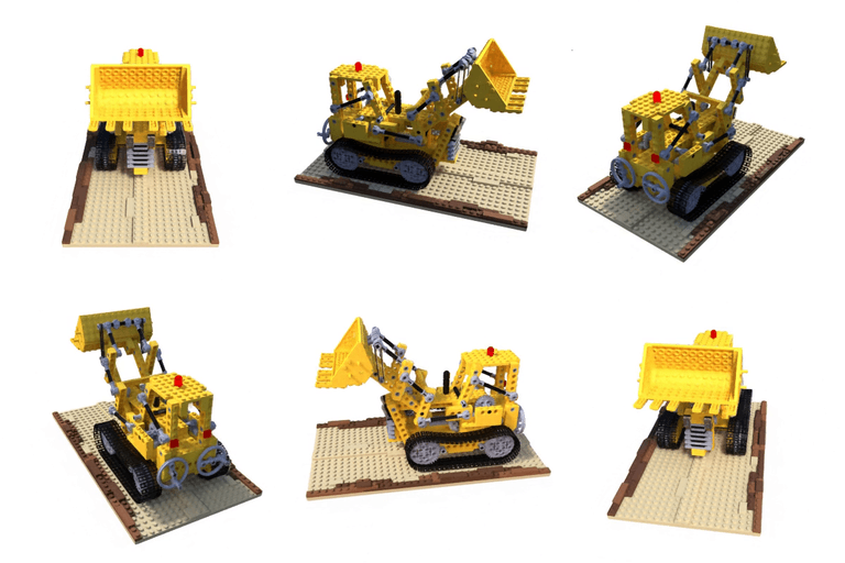
To optimize a low-res Lego NeRF:
python run_nerf.py --config config_lego.txt
After 200k iterations, you should get a video like this:
Rendering a NeRF
Run
bash download_example_weights.sh
to get a pretrained high-res NeRF for the Fern dataset. Now you can use render_demo.ipynb to render new views.
Replicating the paper results
The example config files run at lower resolutions than the quantitative/qualitative results in the paper and video. To replicate the results from the paper, start with the config files in paper_configs/. Our synthetic Blender data and LLFF scenes are hosted here and the DeepVoxels data is hosted by Vincent Sitzmann here.
Extracting geometry from a NeRF
Check out extract_mesh.ipynb for an example of running marching cubes to extract a triangle mesh from a trained NeRF network. You'll need the install the PyMCubes package for marching cubes plus the trimesh and pyrender packages if you want to render the mesh inside the notebook:
pip install trimesh pyrender PyMCubes
Generating poses for your own scenes
Don't have poses?
We recommend using the imgs2poses.py script from the LLFF code. Then you can pass the base scene directory into our code using --datadir <myscene> along with -dataset_type llff. You can take a look at the config_fern.txt config file for example settings to use for a forward facing scene. For a spherically captured 360 scene, we recomment adding the --no_ndc --spherify --lindisp flags.
Already have poses!
In run_nerf.py and all other code, we use the same pose coordinate system as in OpenGL: the local camera coordinate system of an image is defined in a way that the X axis points to the right, the Y axis upwards, and the Z axis backwards as seen from the image.
Poses are stored as 3x4 numpy arrays that represent camera-to-world transformation matrices. The other data you will need is simple pinhole camera intrinsics (hwf = [height, width, focal length]) and near/far scene bounds. Take a look at our data loading code to see more.
Citation
@inproceedings{mildenhall2020nerf,
  title={NeRF: Representing Scenes as Neural Radiance Fields for View Synthesis},
  author={Ben Mildenhall and Pratul P. Srinivasan and Matthew Tancik and Jonathan T. Barron and Ravi Ramamoorthi and Ren Ng},
  year={2020},
  booktitle={ECCV},
}
Top Related Projects
NeRF (Neural Radiance Fields) and NeRF in the Wild using pytorch-lightning
A PyTorch implementation of NeRF (Neural Radiance Fields) that reproduces the results.
Instant neural graphics primitives: lightning fast NeRF and more
PyTorch3D is FAIR's library of reusable components for deep learning with 3D data
Google Research
Plenoxels: Radiance Fields without Neural Networks
Convert  designs to code with AI

Introducing Visual Copilot: A new AI model to turn Figma designs to high quality code using your components.
Try Visual Copilot