pixel-nerf

PixelNeRF Official Repository

1,386

196

1,386

View on GitHub

Top Related Projects

pytorch3d

8,643

PyTorch3D is FAIR's library of reusable components for deep learning with 3D data

nerf

9,767

Code release for NeRF (Neural Radiance Fields)

nerf-pytorch

5,359

A PyTorch implementation of NeRF (Neural Radiance Fields) that reproduces the results.

instant-ngp

15,796

Instant neural graphics primitives: lightning fast NeRF and more

nerf_pl

2,700

NeRF (Neural Radiance Fields) and NeRF in the Wild using pytorch-lightning

Quick Overview

Pixel-NeRF is a neural rendering framework that enables 3D view synthesis from sparse 2D images. It combines the principles of Neural Radiance Fields (NeRF) with a pixel-aligned feature representation, allowing for efficient rendering of novel views without requiring per-scene optimization.

Pros

Fast inference: Can generate novel views in real-time without per-scene training
Generalizes well: Works across different object categories and scenes
Sparse input: Requires only a few input images to generate high-quality novel views
Flexible architecture: Can be adapted for various tasks like 3D reconstruction and pose estimation

Cons

Computational resources: Requires significant GPU memory for training and inference
Limited resolution: Output quality may degrade for very high-resolution images
Dependency on training data: Performance can vary based on the diversity and quality of the training dataset
Complexity: Implementation and fine-tuning can be challenging for newcomers to neural rendering

Code Examples

Loading a pre-trained model:

from pixel_nerf.models import PixelNeRF

model = PixelNeRF.load_from_checkpoint("path/to/checkpoint.ckpt")

Rendering a novel view:

import torch

source_images = torch.rand(1, 3, 3, 256, 256)  # (B, V, C, H, W)
source_poses = torch.rand(1, 3, 4, 4)  # (B, V, 4, 4)
target_pose = torch.rand(1, 4, 4)  # (B, 4, 4)

novel_view = model.render_novel_view(source_images, source_poses, target_pose)

Training the model:

from pixel_nerf.trainer import PixelNeRFTrainer

trainer = PixelNeRFTrainer(
    model=model,
    train_dataset=train_dataset,
    val_dataset=val_dataset,
    num_epochs=100,
    batch_size=4,
    lr=1e-4
)

trainer.train()

Getting Started

Install the required dependencies:

pip install torch torchvision pytorch3d

Clone the repository:

git clone https://github.com/sxyu/pixel-nerf.git
cd pixel-nerf

Install the package:
```
pip install -e .
```
Download pre-trained models:
```
sh scripts/download_model.sh
```

Run inference on a sample image:

from pixel_nerf.models import PixelNeRF
from pixel_nerf.utils import load_image, render_image

model = PixelNeRF.load_from_checkpoint("checkpoints/srn_cars.ckpt")
image = load_image("path/to/image.png")
novel_view = render_image(model, image)
novel_view.save("output.png")

Competitor Comparisons

pytorch3d

8,643

PyTorch3D is FAIR's library of reusable components for deep learning with 3D data

Pros of PyTorch3D

Comprehensive 3D deep learning library with a wide range of functionalities
Backed by Facebook Research, ensuring regular updates and support
Integrates seamlessly with PyTorch ecosystem

Cons of PyTorch3D

Steeper learning curve due to its extensive feature set
May be overkill for simpler 3D rendering tasks
Requires more computational resources for some operations

Code Comparison

PyTorch3D example:

import torch
from pytorch3d.structures import Meshes
from pytorch3d.renderer import Textures

verts = torch.randn(4, 3)
faces = torch.tensor([[0, 1, 2], [1, 2, 3]])
mesh = Meshes(verts=[verts], faces=[faces])

Pixel-NeRF example:

import torch
from models import make_model

model = make_model(args)
model.load_weights(args)
out = model(pixels, poses, focal)

PyTorch3D offers a more comprehensive set of tools for 3D operations, while Pixel-NeRF focuses specifically on neural radiance fields. PyTorch3D is better suited for complex 3D tasks, whereas Pixel-NeRF excels in novel view synthesis using NeRF techniques.

nerf

9,767

Code release for NeRF (Neural Radiance Fields)

Pros of NeRF

Original implementation of the Neural Radiance Fields technique
Highly cited and influential in the field of novel view synthesis
Extensive documentation and explanations in the repository

Cons of NeRF

Slower training and inference times
Limited to static scenes and requires dense input views

Code Comparison

NeRF:

def raw2outputs(raw, z_vals, rays_d, raw_noise_std=0, white_bkgd=False):
    raw2alpha = lambda raw, dists, act_fn=F.relu: 1.-torch.exp(-act_fn(raw)*dists)
    dists = z_vals[...,1:] - z_vals[...,:-1]
    dists = torch.cat([dists, torch.Tensor([1e10]).expand(dists[...,:1].shape)], -1)
    dists = dists * torch.norm(rays_d[...,None,:], dim=-1)

Pixel-NeRF:

def raw2outputs(raw, z_vals, rays_d, raw_noise_std=0, white_bkgd=False):
    rgb = torch.sigmoid(raw[..., :3])
    sigma_a = F.relu(raw[..., 3])
    alpha = 1. - torch.exp(-sigma_a * (z_vals[..., 1:] - z_vals[..., :-1]))
    weights = alpha * torch.cumprod(torch.cat([torch.ones_like(alpha[:, :1]), 1.-alpha + 1e-10], -1), -1)[:, :-1]

nerf-pytorch

5,359

A PyTorch implementation of NeRF (Neural Radiance Fields) that reproduces the results.

Pros of nerf-pytorch

Simpler implementation, making it easier to understand and modify
More closely follows the original NeRF paper, providing a baseline implementation
Includes a colab notebook for quick experimentation

Cons of nerf-pytorch

Limited features compared to pixel-nerf
Less optimized for performance and memory usage
Lacks support for more advanced NeRF variants

Code Comparison

pixel-nerf:

class PixelNeRF(nn.Module):
    def __init__(self, conf):
        super().__init__()
        self.encoder = ImageEncoder(conf)
        self.nerf = NeRF(conf)

    def forward(self, x, rays):
        features = self.encoder(x)
        return self.nerf(rays, features)

nerf-pytorch:

class NeRF(nn.Module):
    def __init__(self, D=8, W=256, input_ch=3, input_ch_views=3, output_ch=4, skips=[4], use_viewdirs=False):
        super(NeRF, self).__init__()
        self.D = D
        self.W = W
        self.input_ch = input_ch
        self.input_ch_views = input_ch_views
        self.skips = skips
        self.use_viewdirs = use_viewdirs
        
        self.pts_linears = nn.ModuleList(
            [nn.Linear(input_ch, W)] + [nn.Linear(W, W) if i not in self.skips else nn.Linear(W + input_ch, W) for i in range(D-1)])

instant-ngp

15,796

Instant neural graphics primitives: lightning fast NeRF and more

Pros of instant-ngp

Significantly faster rendering and training times
Supports real-time rendering of complex 3D scenes
Utilizes GPU acceleration for improved performance

Cons of instant-ngp

Requires more powerful hardware for optimal performance
Less flexible in terms of input data formats
Steeper learning curve for implementation and customization

Code Comparison

pixel-nerf

model = PixelNeRF(...)
rays = get_rays(...)
rgb, depth = model(rays)

instant-ngp

NGP ngp;
ngp.training_step(stream, inputs, ground_truth);
ngp.render(stream, camera_matrix, focal_length, output);

Key Differences

pixel-nerf is implemented in Python using PyTorch, while instant-ngp is written in C++ with CUDA
instant-ngp uses hash-based encoding for faster rendering, whereas pixel-nerf relies on traditional NeRF architecture
pixel-nerf focuses on generalizing to novel views of unseen objects, while instant-ngp prioritizes speed and real-time performance

Use Cases

pixel-nerf: Better suited for research and experimentation with novel view synthesis
instant-ngp: Ideal for applications requiring real-time rendering and interactive 3D scene exploration

google-research

33,785

Google Research

Pros of google-research

Broader scope, covering various research areas and projects
Regularly updated with new research and implementations
Backed by Google, ensuring high-quality and cutting-edge research

Cons of google-research

Less focused on a specific topic, potentially overwhelming for users
May require more effort to navigate and find relevant information
Some projects might be less maintained or documented than others

Code comparison

pixel-nerf:

def forward(self, xyz, view_dir):
    input_pts = torch.cat([xyz, view_dir], dim=-1)
    h = input_pts
    for i, l in enumerate(self.pts_linears):
        h = self.pts_linears[i](h)
        h = F.relu(h)
    outputs = self.output_linear(h)
    return outputs

google-research (example from BERT):

def create_model(bert_config, is_training, input_ids, input_mask, segment_ids,
                 labels, num_labels, use_one_hot_embeddings):
  model = modeling.BertModel(
      config=bert_config,
      is_training=is_training,
      input_ids=input_ids,
      input_mask=input_mask,
      token_type_ids=segment_ids,
      use_one_hot_embeddings=use_one_hot_embeddings)

nerf_pl

2,700

NeRF (Neural Radiance Fields) and NeRF in the Wild using pytorch-lightning

Pros of nerf_pl

Implements multiple NeRF variants, offering more flexibility and options for experimentation
Provides a comprehensive training pipeline with support for distributed training
Includes detailed documentation and examples for easier setup and usage

Cons of nerf_pl

May have a steeper learning curve due to its more complex architecture
Potentially higher computational requirements for training and inference

Code Comparison

pixel-nerf:

class PixelNeRFNet(nn.Module):
    def __init__(self, conf):
        super().__init__()
        self.encoder = ImageEncoder(conf)
        self.nerf = NeRF(conf)

    def forward(self, x):
        feat = self.encoder(x)
        return self.nerf(feat)

nerf_pl:

class NeRFModel(LightningModule):
    def __init__(self, hparams):
        super().__init__()
        self.nerf = NeRF(hparams)
        self.loss = MSELoss()

    def forward(self, rays, ts):
        return self.nerf(rays, ts)

The code snippets show that pixel-nerf uses a separate encoder and NeRF module, while nerf_pl integrates the NeRF model directly into a PyTorch Lightning module for easier training and deployment.

Convert designs to code with AI

Introducing Visual Copilot: A new AI model to turn Figma designs to high quality code using your components.

Try Visual Copilot

README

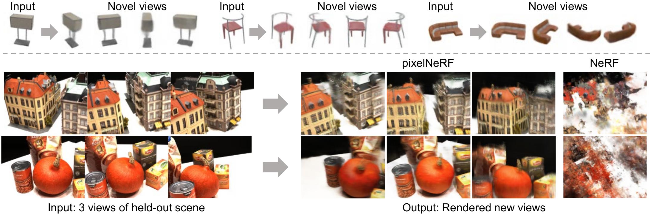
pixelNeRF: Neural Radiance Fields from One or Few Images

Alex Yu, Vickie Ye, Matthew Tancik, Angjoo Kanazawa
UC Berkeley

arXiv: http://arxiv.org/abs/2012.02190

This is the official repository for our paper, pixelNeRF, pending final release. The two object experiment is still missing. Several features may also be added.

Environment setup

To start, we prefer creating the environment using conda:

conda env create -f environment.yml
conda activate pixelnerf

Please make sure you have up-to-date NVIDIA drivers supporting CUDA 10.2 at least.

Alternatively use pip -r requirements.txt.

Getting the data

For the main ShapeNet experiments, we use the ShapeNet 64x64 dataset from NMR https://s3.eu-central-1.amazonaws.com/avg-projects/differentiable_volumetric_rendering/data/NMR_Dataset.zip (Hosted by DVR authors)
- For novel-category generalization experiment, a custom split is needed. Download the following script: https://drive.google.com/file/d/1Uxf0GguAUTSFIDD_7zuPbxk1C9WgXjce/view?usp=sharing place the said file under NMR_Dataset and run python genlist.py in the said directory. This generates train/val/test lists for the experiment. Note for evaluation performance reasons, test is only 1/4 of the unseen categories.
The remaining datasets may be found in https://drive.google.com/drive/folders/1PsT3uKwqHHD2bEEHkIXB99AlIjtmrEiR?usp=sharing
- Custom two-chair multi_chair_{train/val/test}.zip. Download splits into a parent directory and pass the parent directory path to training command.
  - To render out your own dataset, feel free to use our script in scripts/render_shapenet.py. See scripts/README.md for installation instructions.
- DTU (4x downsampled, rescaled) in DVR's DTU format dtu_dataset.zip
- SRN chair/car (128x128) srn_*.zip needed for single-category exps. Note the car set is a re-rendered version provided by Vincent Sitzmann

While we could have used a common data format, we chose to keep DTU and ShapeNet (NMR) datasets in DVR's format and SRN data in the original SRN format. Our own two-object data is in NeRF's format. Data adapters are built into the code.

Running the model (video generation)

The main implementation is in the src/ directory, while evalutation scripts are in eval/.

First, download all pretrained weight files from https://drive.google.com/file/d/1UO_rL201guN6euoWkCOn-XpqR2e8o6ju/view?usp=sharing. Extract this to <project dir>/checkpoints/, so that <project dir>/checkpoints/dtu/pixel_nerf_latest exists.

ShapeNet Multiple Categories (NMR)

Download NMR ShapeNet renderings (see Datasets section, 1st link)
Run using
- python eval/gen_video.py -n sn64 --gpu_id <GPU(s)> --split test -P '2' -D <data_root>/NMR_Dataset -S 0
- For unseen category generalization: python eval/gen_video.py -n sn64_unseen --gpu_id=<GPU(s)> --split test -P '2' -D <data_root>/NMR_Dataset -S 0

Replace <GPU(s)> with desired GPU id(s), space separated for multiple. Replace -S 0 with -S <object_id> to run on a different ShapeNet object id. Replace -P '2' with -P '<number>' to use a different input view. Replace --split test with --split train | val to use different data split. Append -R=20000 if running out of memory.

Result will be at visuals/sn64/videot<object_id>.mp4 or visuals/sn64_unseen/videot<object_id>.mp4. The script will also print the path.

Pre-generated results for all ShapeNet objects with comparison may be found at https://www.ocf.berkeley.edu/~sxyu/ZG9yaWF0aA/pixelnerf/cross_v2/

ShapeNet Single-Category (SRN)

Download SRN car (or chair) dataset from Google drive folder in Datasets section. Extract to <srn data dir>/cars_<train | test | val>
python eval/gen_video.py -n srn_car --gpu_id=<GPU (s)> --split test -P '64 104' -D <srn data dir>/cars -S 1

Use -P 64 for 1-view (view numbers are from SRN). The chair set case is analogous (replace car with chair). Our models are trained with random 1/2 views per batch during training. This seems to degrade performance especially for 1-view. It may be preferrable to use a fixed number of views instead.

DTU

Make sure you have downloaded the pretrained weights above.

Download DTU dataset from Google drive folder in Datasets section. Extract to some directory, to get: <data_root>/rs_dtu_4
Run using python eval/gen_video.py -n dtu --gpu_id=<GPU(s)> --split val -P '22 25 28' -D <data_root>/rs_dtu_4 -S 3 --scale 0.25

Replace <GPU(s)> with desired GPU id(s). Replace -S 3 with -S <scene_id> to run on a different scene. This is not DTU scene number but 0-14 in the val set. Remove --scale 0.25 to render at full resolution (quite slow).

Result will be at visuals/dtu/videov<scene_id>.mp4. The script will also print the path.

Note that for DTU, I only use train/val sets, where val is used for test. This is due to the very small size of the dataset. The model overfits to the train set significantly during training.

Real Car Images

Note: requires PointRend from detectron2. Install detectron2 by following https://github.com/facebookresearch/detectron2/blob/master/INSTALL.md.

Make sure you have downloaded the pretrained weights above.

Download any car image. Place it in <project dir>/input. Some example images are shipped with the repo. The car should be fully visible.
Run the preprocessor script: python scripts/preproc.py. This saves input/*_normalize.png. If the result is not reasonable, PointRend didn't work; please try another imge.
Run python eval/eval_real.py. Outputs will be in <project dir>/output

The Stanford Car dataset contains many example car images: https://ai.stanford.edu/~jkrause/cars/car_dataset.html. Note the normalization heuristic has been slightly modified compared to the paper. There may be some minor differences. You can pass -e -20 to eval_real.py to set the elevation higher in the generated video.

Overview of flags

Generally, all scripts in the project take the following flags

-n <expname>: experiment name, matching checkpoint directory name
-D <datadir>: dataset directory. To save typing, you can set a default data directory for each expname in expconf.conf under datadir. For SRN/multi_obj datasets with separate directories e.g. path/cars_train, path/cars_val, put -D path/cars.
--split <train | val | test>: data set split
-S <subset_id>: scene or object id to render
--gpu_id <GPU(s)>: GPU id(s) to use, space delimited. All scripts except calc_metrics.py are parallelized. If not specified, uses GPU 0. Examples: --gpu_id=0 or --gpu_id='0 1 3'.
-R <sz>: Batch size of rendered rays per object. Default is 50000 (eval) and 128 (train); make it smaller if you run out of memory. On large-memory GPUs, you can set it to 100000 for eval.
-c <conf/*.conf>: config file. Automatically inferred for the provided experiments from the expname. Thus the flag is only required when working with your own expnames. You can associate a config file with any additional expnames in the config section of <project root>/expconf.conf.

Please refer the the following table for a list of provided experiments with associated config and data files:

Name	expname -n	config -c (automatic from expconf.conf)	Data file	data dir -D
ShapeNet category-agnostic	sn64	conf/exp/sn64.conf	NMR_Dataset.zip (from AWS)	path/NMR_Dataset
ShapeNet unseen category	sn64_unseen	conf/exp/sn64_unseen.conf	NMR_Dataset.zip (from AWS) + genlist.py	path/NMR_Dataset
SRN chairs	srn_chair	conf/exp/srn.conf	srn_chairs.zip	path/chairs
SRN cars	srn_car	conf/exp/srn.conf	srn_cars.zip	path/cars
DTU	dtu	conf/exp/dtu.conf	dtu_dataset.zip	path/rs_dtu_4
Two chairs	mult_obj	conf/exp/mult_obj.conf	multi_chair_{train/val/test}.zip	path

Quantitative evaluation instructions

All evaluation code is in eval/ directory. The full, parallelized evaluation code is in eval/eval.py.

Approximate Evaluation

The full evaluation can be extremely slow (taking many days), especially for the SRN dataset. Therefore we also provide eval_approx.py for approximate evaluation.

Example python eval/eval_approx.py -D <srn_data>/cars -n srn_car

Add --seed <number> to try a different random seed.

Full Evaluation

Here we provide commands for full evaluation with eval/eval.py. After running this you should also use eval/calc_metrics.py, described in the section below, to obtain final metrics.

Append --gpu_id=<GPUs> to specify GPUs, for example --gpu_id=0 or --gpu_id='0 1 3'. It is highly recommended to use multiple GPUs if possible to finish in reasonable time. We use 4-10 for evaluations as available. Resume-capability is built-in, and you can simply run the command again to resume if the process is terminated.

In all cases, a source-view specification is required. This can be either -P or -L. -P 'view1 view2..' specifies a set of fixed input views. In contrast, -L should point to a viewlist file (viewlist/src_*.txt) which specifies views to use for each object.

Renderings and progress will be saved to the output directory, specified by -O <dirname>.

ShapeNet Multiple Categories (NMR)

Category-agnostic eval python eval/eval.py -D <path>/NMR_Dataset -n sn64 -L viewlist/src_dvr.txt --multicat -O eval_out/sn64
Unseen category eval python eval/eval.py -D <path>/NMR_Dataset -n sn64_unseen -L viewlist/src_gen.txt --multicat -O eval_out/sn64_unseen

ShapeNet Single-Category (SRN)

SRN car 1-view eval python eval/eval.py -D <srn_data>/cars -n srn_car -P '64' -O eval_out/srn_car_1v
SRN car 2-view eval python eval/eval.py -D <srn_data>/cars -n srn_car -P '64 104' -O eval_out/srn_car_2v

The command for chair is analogous (replace car with chair). The input views 64, 104 are taken from SRN. Our method is by no means restricted to using such views.

DTU

1-view python eval/eval.py -D <data>/rs_dtu_4 --split val -n dtu -P '25' -O eval_out/dtu_1v
3-view python eval/eval.py -D <data>/rs_dtu_4 --split val -n dtu -P '22 25 28' -O eval_out/dtu_3v
6-view python eval/eval.py -D <data>/rs_dtu_4 --split val -n dtu -P '22 25 28 40 44 48' -O eval_out/dtu_6v
9-view python eval/eval.py -D <data>/rs_dtu_4 --split val -n dtu -P '22 25 28 40 44 48 0 8 13' -O eval_out/dtu_9v

In training, we always provide 3-views, so the improvement with more views is limited.

Final Metric Computation

The above computes PSNR and SSIM without quantization. The final metrics we report in the paper use the rendered images saved to disk, and also includes LPIPS + category breakdown. To do so run the eval/calc_metrics.py, as in the following examples

NMR ShapeNet experiment: python eval/calc_metrics.py -D <data dir>/NMR_Dataset -O eval_out/sn64 -F dvr --list_name 'softras_test' --multicat --gpu_id=<GPU>
SRN car 2-view: python eval/calc_metrics.py -D <srn data dir>/cars -O eval_out/srn_car_2v -F srn --gpu_id=<GPU> (warning: untested after changes)
DTU: python eval/calc_metrics.py -D <data dir>/rs_dtu_4/DTU -O eval_out/dtu_3v -F dvr --list_name 'new_val' --exclude_dtu_bad --dtu_sort

Adjust -O according to the -O flag of the eval.py command. (Note: Currently this script has an ugly standalone argument parser.) This should print a metric summary like the following

psnr 26.799268696042386
ssim 0.9102204550379002
lpips 0.10784384977842876
WROTE eval_sn64/all_metrics.txt
airplane     psnr: 29.756697 ssim: 0.946906 lpips: 0.084329 n_inst: 809
bench        psnr: 26.351427 ssim: 0.911226 lpips: 0.116299 n_inst: 364
cabinet      psnr: 27.720198 ssim: 0.910426 lpips: 0.104584 n_inst: 315
car          psnr: 27.579590 ssim: 0.942079 lpips: 0.094841 n_inst: 1500
chair        psnr: 23.835303 ssim: 0.857738 lpips: 0.145518 n_inst: 1356
display      psnr: 24.217023 ssim: 0.867284 lpips: 0.129138 n_inst: 219
lamp         psnr: 28.579184 ssim: 0.912794 lpips: 0.113561 n_inst: 464
loudspeaker  psnr: 24.435302 ssim: 0.855195 lpips: 0.140653 n_inst: 324
rifle        psnr: 30.597488 ssim: 0.968040 lpips: 0.065629 n_inst: 475
sofa         psnr: 26.944224 ssim: 0.907861 lpips: 0.116114 n_inst: 635
table        psnr: 25.591960 ssim: 0.898314 lpips: 0.098103 n_inst: 1702
telephone    psnr: 27.128039 ssim: 0.921897 lpips: 0.097074 n_inst: 211
vessel       psnr: 29.180307 ssim: 0.938936 lpips: 0.110670 n_inst: 388
---
total        psnr: 26.799269 ssim: 0.910220 lpips: 0.107844

Training instructions

Training code is in train/ directory, specifically train/train.py.

Example for training to DTU: python train/train.py -n dtu_exp -c conf/exp/dtu.conf -D <data dir>/rs_dtu_4 -V 3 --gpu_id=<GPU> --resume
Example for training to SRN cars, 1 view: python train/train.py -n srn_car_exp -c conf/exp/srn.conf -D <srn data dir>/cars --gpu_id=<GPU> --resume
Example for training to ShapeNet multi-object, 2 view: python train/train.py -n multi_obj -c conf/exp/multi_obj.conf -D <parent dir of splits> --gpu_id=<GPU> --resume

Additional flags

--resume to resume from checkpoint, if available. Usually just pass this to be safe.
-V <number> to specify number of input views to train with. Default is 1.
- -V 'numbers separated by space' to use random number of views per batch. This does not work so well in our experience but we use it for SRN experiment.
-B <number> batch size of objects, default 4
--lr <learning rate>, --epochs <number of epochs>
--no_bbox_step <number> to specify iteration after which to stop using bounding-box sampling. Set to 0 to disable.

If the checkpoint becomes corrupted for some reason (e.g. if process crashes when saving), a backup is saved to checkpoints/<expname>/pixel_nerf_backup. To avoid having to specify -c, -D each time, edit <project root>/expconf.conf and add rows for your expname in the config and datadir sections.

Log files and visualizations

View logfiles with tensorboard --logdir <project dir>/logs/<expname>. Visualizations are written to <project dir>/visuals/<expname>/<epoch>_<batch>_vis.png. They are of the form

Top coarse, bottom fine (1 row if fine sample disabled)
Left-to-right: input-views, depth, output, alpha.

BibTeX

@inproceedings{yu2021pixelnerf,
      title={{pixelNeRF}: Neural Radiance Fields from One or Few Images},
      author={Alex Yu and Vickie Ye and Matthew Tancik and Angjoo Kanazawa},
      year={2021},
      booktitle={CVPR},
}

Acknowledgements

Parts of the code were based on from kwea123's NeRF implementation: https://github.com/kwea123/nerf_pl. Some functions are borrowed from DVR https://github.com/autonomousvision/differentiable_volumetric_rendering and PIFu https://github.com/shunsukesaito/PIFu

Top Related Projects

Convert designs to code with AI

Introducing Visual Copilot: A new AI model to turn Figma designs to high quality code using your components.

Try Visual Copilot